Step 1A: Let’s first consider the path‑graph case

When solving a competitive programming problem and the solution isn’t clear, a good strategy is to consider simpler cases. In Steps 1A, 1B, and 1C, we take the most primitive case: the path graph (that is, \(M = N - 1\) with edges \(1 \to 2, 2 \to 3, \dots, (N-1) \to N\)).

Let us look at some examples.

Example 1
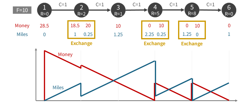
Take \(N = 6, F = 10, C_i = 1, R = (0, 2, 1, 5, 8, 0)\). The optimal solution is illustrated below.

Observe the result:

• At airport \(3\), you pass through without exchanging.
  
• At airport \(5\), you exchange all the miles you have.
  
• At airports \(2\) and \(4\), you exchange just enough miles so that your remaining money will exactly last until the next exchange.
  

Example 2
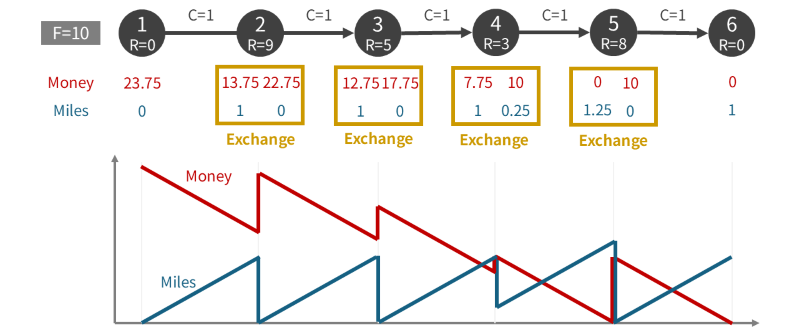
Take \(N = 6, F = 10, C_i = 1, R = (0, 9, 5, 3, 8, 0)\). The optimal solution is illustrated below.

Observe the result:

• At airports \(2, 3, 5\), you exchange all the miles you have.
  
• At airport \(4\), you exchange just enough miles so that your remaining money will exactly last until the next exchange.
  

---

Step 1B: Exploring the structure of the optimal solution

These two examples suggest the following property of the optimal solution. Does it hold in general?

Property
When you perform an exchange, you either
1. exchange all the miles you currently have (Type A), or
2. exchange just enough miles so that your remaining money will be exactly zero upon arrival at the next exchange point (Type B).

In fact, this property always holds. Intuitively, if you ever perform an exchange that is neither Type A nor Type B, you could shift a small amount of miles \(\varepsilon\) between that airport and the next one in whichever direction increases your final money.

Rigorous proof

Suppose at some airport \(x\) you perform an exchange that is neither Type A nor Type B. Let \(y\) be the next airport, and choose a sufficiently small \(\varepsilon>0\).

• Case \(R_x > R_y\): Increase the miles exchanged at \(x\) by \(\varepsilon\), and decrease the miles exchanged at \(y\) by \(\varepsilon\). Your miles at \(y\) remain the same, but your money increases by \(\varepsilon(R_x - R_y)>0\).
• Case \(R_x < R_y\): Decrease the miles exchanged at \(x\) by \(\varepsilon\), and increase the miles exchanged at \(y\) by \(\varepsilon\). Again, your miles at \(y\) stay the same, and your money increases by \(\varepsilon(R_y - R_x)>0\).

The first adjustment is feasible because not all miles are exchanged at airport \(x\), and the second adjustment is feasible because the exchange at airport \(x\) ensures that you have some money left at the next exchange point.

The only subtle case is \(R_x = R_y\), but by imposing a tie‑breaker such as “among the solutions with the same initial money, the one that postpones exchanges is better,” one direction strictly improves.

Hence, the Property holds in any optimal solution.

Here, Type A means your miles drop to 0 when departing that airport, and Type B means your money drops to 0 upon arriving at the next airport. We can visualize this:

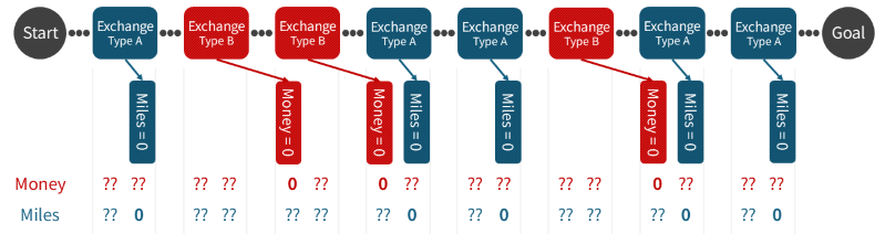
From this, we see that you never perform two consecutive exchanges that are neither zero‑money nor zero‑miles. More concretely:

1. Type A → Type A: From a zero‑miles state to another zero‑miles state, there are no exchanges at intermediate airports.
2. Type A → Type B: From a zero-miles state to a zero-money state, there is exactly one exchange at an intermediate airport.
3. Type B → Type A: From a zero-money state to a zero-miles state, the transition happens at the same airport.
4. Type B → Type B: From a zero-money state to another zero-money state, there are no exchanges at intermediate airports.

---

Step 1C: Solving the path case with dynamic programming (DP)

We now consider the decision problem: given an initial money amount \(x\), can you reach airport \(N\)? The answer to the original problem is found by binary searching on \(x\).

From Step 1B, you perform exchanges while passing through zero‑miles or zero‑money states. Define:

• \(\mathrm{dp}_1[i]\): Maximum money you can have when departing airport \(i\) with \(0\) miles.
  
• \(\mathrm{dp}_2[i]\): Maximum miles you can have when arriving at airport \(i\) with \(0\) money.
  

The transitions \(\mathrm{dp}_1[j] \to \mathrm{dp}_1[i]\), \(\mathrm{dp}_1[j] \to \mathrm{dp}_2[i]\), \(\mathrm{dp}_2[j] \to \mathrm{dp}_1[i]\), and \(\mathrm{dp}_2[j] \to \mathrm{dp}_2[i]\) correspond to the above cases Type A → Type A, Type A → Type B, Type B → Type A, and Type B → Type B, respectively. Among these, only \(\mathrm{dp}_1[j] \to \mathrm{dp}_2[i]\) requires an exchange at some intermediate airport \(k\) (\(j<k<i\)). We must try all \(k\), so it takes \(O(N^3)\) time to compute all DP values.

Therefore, the path case can be solved in \(O(N^3 \log \frac{1}{\varepsilon})\) time (\(\varepsilon=10^{-6}\) is the permitted error).

---

Step 2A: Extending to general graphs

In a general graph, the same exchange properties hold, so we again want \(\mathrm{dp}_1[i]\) and \(\mathrm{dp}_2[i]\). However, unlike the path case, we do not know an order in which we compute them (actually, for a graph with cycles we cannot compute them in a fixed order).

Instead, introduce the number of exchanges \(t\) and use a Bellman–Ford–style DP:

• \(\mathrm{dp}_1[t][i]\): Maximum money at departure from airport \(i\) with \(0\) miles, after \(t\) exchanges.
  
• \(\mathrm{dp}_2[t][i]\): Maximum miles at arrival at airport \(i\) with \(0\) money, after \(t\) exchanges.
  

Now, we can compute them in ascending order of \(t\). Since it is never optimal to exchange more than once at the same airport (after visiting other airports and coming back), we only need the values for \(t\le N\). Computing this DP takes \(O(N^4)\) time, so this solves the general graph case in \(O(N^4 \log \frac{1}{\varepsilon})\) time.

(The computation of this DP involves calculating the minimum cost to go from an airport to another without intermediate exchanges, which can be precomputed by Floyd–Warshall in \(O(N^3)\) time.)

---

Step 2B: DP optimization 1 — from Bellman–Ford to Dijkstra

The Bellman–Ford style above is slow. Can we do it Dijkstra‑style?

To do so, we need an order in which we “fix” the values of \(\mathrm{dp}_1[i], \mathrm{dp}_2[i]\) and then update unfixed \(\mathrm{dp}_1[j], \mathrm{dp}_2[j]\) by transitions \(\mathrm{dp}_{?}[i] \to \mathrm{dp}_{?}[j]\).

A convenient property is:

Property: During the process, (money) + F × (miles) is non-increasing.

Proof

• When traveling along route \(j\), money decreases by \(C_j \times F\) and miles increase by \(C_j\), so (money) + F × (miles) is unchanged.
• When exchanging \(d\) miles at airport \(i\), money increases by \(d \times R_i\); since \(R_i<F\), (money) + F × (miles) decreases.

Thus, we can fix DP states in descending order of (money) + F × (miles), that is, descending order of \(\mathrm{dp}_1[i]\) or \(F \times \mathrm{dp}_2[i]\). This reduces DP computation to \(O(N^3)\).

Hence, the general graph case is solved in \(O(N^3 \log \frac{1}{\varepsilon})\) time.

---

Step 2C: DP optimization 2 — working backwards

Finally, we remove the binary search factor by defining DP from airport \(N\) backwards:

• \(\mathrm{dp}'_1[i]\): Minimum money needed when departing airport \(i\) with \(0\) miles to reach airport \(N\).
  
• \(\mathrm{dp}'_2[i]\): Minimum miles needed when arriving at airport \(i\) with \(0\) money to reach airport \(N\).
  

We compute these in the opposite direction from what we did above. For example, for the transition Type A → Type A, we compute: “to end up with \(\mathrm{dp}'_1[i]\) money + \(0\) miles when departing airport \(i\), how much money (+ \(0\) miles) do we need to have when departing airport \(j\)?” (The answer is \(\max(\mathrm{dp}'[i] - d \times R_i, 0) + F \times d\), where \(d\) is the distance from \(j\) to \(i\) in the graph.) We run a Dijkstra‑like process, fixing states in ascending order of \(\mathrm{dp}'_1[i]\) or \(F \times \mathrm{dp}'_2[i]\).

The answer to the problem is \(\mathrm{dp}'_1[1]\). This yields an \(O(N^3)\) algorithm without binary search.

---

Sample implementation (C++)

#include <vector>
#include <iostream>
#include <algorithm>
using namespace std;

const int INF = 1012345678;

// Function to compute all‑pairs shortest paths using the Floyd–Warshall algorithm
vector<vector<int> > warshall_floyd(int N, vector<vector<int> > C) {
    for (int i = 0; i < N; i++) {
        C[i][i] = 0;
    }
    for (int i = 0; i < N; i++) {
        for (int j = 0; j < N; j++) {
            for (int k = 0; k < N; k++) {
                C[j][k] = min(C[j][k], C[j][i] + C[i][k]);
            }
        }
    }
    return C;
}

// Function to solve the problem
double solve(int N, int F, const vector<vector<int> >& C, const vector<int>& R) {
    // step #1. Dijkstra‑like preparation
    vector<vector<int> > d = warshall_floyd(N, C);  // all‑pairs shortest distances
    vector<double> dp1(N, 1.0e+99), dp2(N, 1.0e+99);  // DP values
    vector<bool> used1(N, false), used2(N, false);    // fixed‑state flags
    dp1[N - 1] = 0.0;

    // step #2. Dijkstra‑like algorithm
    while (true) {
        // pick the next state to fix
        double opt = 1.0e+99;
        int tp = -1, u = -1;
        for (int i = 0; i < N; i++) {
            if (!used1[i] && opt > dp1[i]) {
                opt = dp1[i];
                tp = 1;
                u = i;
            }
            if (!used2[i] && opt > dp2[i] * F) {
                opt = dp2[i] * F;
                tp = 2;
                u = i;
            }
        }
        // no more states to fix
        if (tp == -1) {
            break;
        }
        // fix the chosen state
        if (tp == 1) {
            used1[u] = true;
        } else {
            used2[u] = true;
        }
        // Transition: dp2[u] <- dp1[u]
        if (tp == 1) {
            if (!used2[u] && R[u] != 0) {
                dp2[u] = min(dp2[u], dp1[u] / R[u]);
            }
        }
        // Transition: dp1[j] <- dp1[u]
        if (tp == 1) {
            for (int j = 0; j < N; j++) {
                if (!used1[j] && d[j][u] != INF) {
                    double x = d[j][u] * F + max(dp1[u] - d[j][u] * R[u], 0.0);
                    dp1[j] = min(dp1[j], x);
                }
            }
        }
        // Transition: dp2[j] <- dp2[u]
        if (tp == 2) {
            for (int j = 0; j < N; j++) {
                if (!used2[j] && d[j][u] != INF && R[j] != 0) {
                    double x = double(d[j][u] * F) / R[j] + max(dp2[u] - d[j][u], 0.0);
                    dp2[j] = min(dp2[j], x);
                }
            }
        }
        // Transition: dp1[k] <- dp2[u]
        if (tp == 2) {
            for (int j = 0; j < N; j++) {
                if (d[j][u] != INF) {
                    if (dp2[u] <= d[j][u]) {
                        if (!used1[j]) {
                            double x = d[j][u] * F;
                            dp1[j] = min(dp1[j], x);
                        }
                    } else if (R[j] != 0) {
                        // Case with an intermediate airport: go k -> j -> u (j is the intermediate)
                        for (int k = 0; k < N; k++) {
                            if (!used1[k] && dp2[u] <= d[j][u] + d[k][j]) {
                                double diff = (d[j][u] + d[k][j]) - dp2[u];
                                double money = d[j][u] * F - diff * R[j];
                                if (money > 0) {
                                    money += d[k][j] * F;
                                    dp1[k] = min(dp1[k], money);
                                }
                            }
                        }
                    }
                }
            }
        }
    }

    // The answer is dp1[0]
    return dp1[0];
}

int main() {
    cin.tie(nullptr);
    ios::sync_with_stdio(false);
    int TESTCASES;
    cin >> TESTCASES;
    for (int id = 1; id <= TESTCASES; id++) {
        int N, M, F;
        cin >> N >> M >> F;
        vector<vector<int> > C(N, vector<int>(N, INF));
        for (int i = 0; i < M; i++) {
            int a, b, c;
            cin >> a >> b >> c;
            a--; b--;
            C[a][b] = min(C[a][b], c);
        }
        vector<int> R(N);
        for (int i = 0; i < N; i++) {
            cin >> R[i];
        }
        long double ans = solve(N, F, C, R);
        cout.precision(16);
        cout << fixed << ans << '\n';
    }
    return 0;
}

---

Supplement: proof of error bounds

In this problem, we use floating‑point arithmetic to compute the answer, but one can prove the relative error is bounded by \(O(N\varepsilon)\), where \(\varepsilon\) is machine epsilon (e.g., \(2^{-53}\) for double). Each of the four transitions is essentially of the form \(\mathrm{dp}_?[?] \times (\text{positive constant}) + (\text{positive constant})\) (here, “constant” does not depend on the DP values), and such an operation introduces only \(O(\varepsilon)\) relative error.