 /
/ 
実行時間制限: 2 sec / メモリ制限: 1024 MiB
ストーリー
あなたは自動車工場の生産管理部門で働いています。工場では現在、増加する需要に応えるため新しい生産ラインを建設する計画が進んでおり、これが完成すれば生産能力が大幅に向上することが期待されています。
しかし、新ラインの生産能力がどの程度なのかはまだ正確には分かっていません。そこでプログラマであるあなたは、新ラインによってどの程度の需要を満たすことができるのかを調べてみることにしました。
問題文
新ラインには、ひとつながりの長いベルトコンベアがあります。このラインでは車種 1, 2, \dots, M の M 種類の車を生産する予定であり、どの車もこのベルトコンベアに載せて、流れ作業で組み立てます。ベルトコンベアに沿って S 人の作業員が配置されており、流れてきた車に対して部品の取り付けなどの作業を行います。車は T 秒間隔で流れてきます(ただし、後述のベルトコンベアが停止した場合を除く)。
作業員はそれぞれ移動可能な範囲が定められており、その範囲内にある車に対しては作業ができますが、そうでない車に対しては作業ができません。条件を正確に述べるために、ベルトコンベアに沿って実数の座標が設定されていると考えます。ベルトコンベアの進行方向が正の向きです。定式化を簡単にするため、ベルトコンベアは両端に無限に延びていると考えます。作業員に 1, 2, \dots, S と順番に番号を割り振ったとき、作業員 j が作業を行えるのは作業対象の車の座標が閉区間 [x_{j-1}+1, x_j] に含まれるときです(ただし x_0 = 0 < x_1 < \dots < x_S)。すなわち、作業員 j は車の座標が x_{j-1}+1 に達したときにその車に作業を行えるようになり、座標が x_j を超えると作業を行えなくなります。この区間のことを作業ステーション j と呼びます。
車種 i の車に対する作業ステーション j での作業には t_{i,j} 秒かかります。
一人の作業員が同時に複数の車に対して作業を行うことはできません。一つの作業ステーションに複数の車が存在するときは、座標の大きい車の作業を先に行います。
ベルトコンベアは通常、秒速 1 の速さで流れていますが、ある作業ステーションでの作業が間に合わない場合(つまり作業が終わっていない車がその作業ステーションの終端にあるとき)は、その作業が終わるまで一時的に停止します。すべての車は同じベルトコンベアの上に載っているので、停止している間はすべての車の移動が止まります。よって、ベルトコンベアが停止している間は作業を終えた車も次の作業ステーションに移動できないので、停止時間が長いほど生産効率が落ちることになります。
車種 i は一日あたり n_i 台の需要があります。一日の作業時間は限られており、最大で L 秒までしか作業ができません。この制限時間のもとで需要をできるだけ満たす計画を立ててください。
計画は、その日に何台の車を作るかを表す非負整数 K と、長さ K の数列 p_1, p_2, \dots, p_K で表されます。p_k は k 番目に作る車の車種です。ただし車種 i は n_i 台までしか作らないものとします。
入力
入力は以下のフォーマットで与えられます。
M S T L
t_{1, 1} ... t_{1, S}
t_{2, 1} ... t_{2, S}
:
t_{M, 1} ... t_{M, S}
x_1 x_2 ... x_S
n_1 ... n_M
入力される値はすべて整数です。暫定テストとシステムテストに使われるテストケースは以下の条件を満たします。
- (M, S) = (20, 40), (40, 80)
- T = 60
- 1 \le L
- 0 < t_{i,j} (1 \le i \le M, 1 \le j \le S)
- t_{i,1} < x_1, t_{i,j} < x_j - x_{j-1} (1 \le i \le M, 2 \le j \le S)
- T < x_1, T < x_j - x_{j-1} (1 \le i \le M, 2 \le j \le S)
- 1 \le n_i (1 \le i \le M)
- n_1 + n_2 + \dots + n_M = 1000
出力
計画を以下のフォーマットで出力してください。出力が問題文中にある計画の要件を満たさない場合は誤答となります。
K
p_1 p_2 ... p_K
K < n_1 + n_2 + \dots + n_M でも構わないことに注意してください。すなわち、出力する台数が需要数より少なくても誤答とはなりません。
得点
時刻が L に達するかすべての車を完成させるまで生産ラインをシミュレートします(後述)。シミュレーションが終了したときに車 i が m_i 台完成しているとして、得点を以下のように定めます。
- すべての i について m_i = n_i のとき、すべての車が完成する時刻を t として 10^6 \times (2 - {t \over L}) を最も近い整数に丸めた値
- そうでないとき \displaystyle{{10^6 \over M} \sum_{i=1}^M \sqrt{m_i \over n_i}} を最も近い整数に丸めた値
シミュレーション方法
生産ラインのシミュレーションは以下のように行います。現実世界では時刻や車の位置、作業の進み具合は連続的に変化しますが、以下では手続きとして記述する都合上、1 秒単位で離散的に変化させています。
以下の変数を使います。
- b: ベルトコンベアが停止しているか動いているかを表すフラグ
- t: 現在時刻
- y_k: k 番目に作る車の座標
- r(k, j): 作業 (k, j) の進捗。ただし作業 (k, j) とは、k 番目の車の作業ステーション j での作業を指します。
変数への代入は \gets で表します。 また、作業 (k, j) が完了しているとは、r(k, j) = t_{p_k, j} であることとします。
- t \gets 0, y_k \gets -(k-1)\times T, r(k, j) \gets 0 と初期化する。
- t = L となるか、作業 (N, S) が完了するまで以下を繰り返す。
- 「x_j = y_k かつ作業 (k, j) は完了していない」を満たす k, j の組があるなら、b \gets 1 とする。そのような組がないなら b \gets 0 とする。
- 各作業ステーション j について、「k 番目の車は j の作業区間内にあり、作業 (k, j) は未完了である」を満たす k があれば、そのような最小の k について r(k, j) を 1 増やす。そのような k がなければ何もしない。
- b = 0 であれば、すべての k について y_k を 1 増やす。b = 1 なら y_k は変化しない。
- 時刻 t を 1 増やす。
- m_i をこの時点で完成している車種 i の車の数とする。より厳密には、r(k, S) = t_{p_k,S} かつ p_k = i を満たす k の個数を m_i とする。
入力生成方法
暫定テストとシステムテストに使われるテストケースは以下の方法で生成されます。ただし、詳細は一部省略していますので、さらに詳しく知りたい方は testcase_generator.cpp を見てください。
パラメータ
- \alpha = 0.5, 0.7, 0.8 (大きいほど作業時間 t_{i,j} が長くなる)
- \beta = 1.0
- c = 1.0, 1.1 (大きいほど作業ステーションの長さ x_j-x_{j-1}-1 が長くなる)
- d = 0.1
- f = 0, 1 (f = 1 のときは入力に試作品が一台含まれる。作業員は試作品の作業手順には慣れていないため、作業時間が他の車種よりも長くかかることがある)
- s = 3, 4 (M, S などの値を決めるのに使う)
可能な 24 通りの組合せから \alpha = 0.8, c = 1.0 の場合を除いた 20 通りそれぞれについて、5 ケースを生成して暫定テスト、50 ケースを生成してシステムテストのテストケースとします。
システムテスト用のテストケース生成に使用するパラメータ一覧 (parameters_systemtest_onlinejudge.txt; md5=4a1081f7fd143943def4e95c4979b6a6) はコンテスト終了後に公開します。
生成方法の概要
x 以上 y 以下の実数と整数を一様ランダムに生成する関数を、それぞれ \mathrm{rand}(x, y), \mathrm{randint}(x, y) と表す。
- M = 5 \times 2^{s-1}, S = 5 \times 2^s, T = 60, N = 1000 とする。
- t_{i,j} を、T に対して極端に大きな値にならないように決める。(詳細は後述)
- 正の実数 w_i を定める。w_i は車種 i の生産比率と呼ばれる。\sum_j t_{i,j} が大きい i ほど w_i は小さくなる傾向がある。(詳細は後述)
- x_1 = l_1 + 1, x_j = x_{j-1} + l_j + 1 とする。ただし l_j は作業ステーション j の長さであり、l_j = \max(T, \max_i t_{i,j} \times c) と定義される。
- L = \mathrm{round}(\mathrm{rand}(1-d, 1+d) \times (T \times N+x_S)) とする。
- f = 1 の場合、車種 M の車は試作品とする。作業時間を t_{M,j} \gets \mathrm{randint}(t_{M,j}, x_j - x_{j-1} - 1) と変更する。この変更は上記の x_j などを決めた後で行われる。
- n_i は、まず n_i = 1 と初期化し、次の操作を N-M 回繰り返すことで定める。
- 試作品でない車種 i を一つ選び、n_i を 1 増やす。このとき i が選択される確率は w_i に比例する。
t_{i,j}, w_i の定め方の概略を表示
- A = P = 2^s とする。
- S 個の作業ステーションは P 個の区間に分けられる。P 個の区間のそれぞれを工程と呼ぶ。工程は 1, 2, \dots, P で番号付けられる。
- S = 10, P = 3 の場合の分け方の例として次のようなものが考えられる: 工程 1 は作業ステーション 1, 2, 3 からなり、工程 2 は作業ステーション 4, 5, 6 からなり、工程 3 は作業ステーション 7, 8, 9, 10 からなる。
- 車にはいくつかの属性がある。属性には 1, 2, \dots, A の番号が付いている。車種 i ごとにそれが持つ属性の集合をランダム(一様とは限らない)に決める。
- 各属性は工程の作業に影響を与えることがある。具体的には、いくつかの工程に追加の部品の取り付けなどの作業を発生させ、その工程の作業時間を長くする。属性ごとに影響を与える工程(複数の場合もある)とその影響度をランダム(一様とは限らない)に決める。属性 a の工程 p への影響度を X_{a,p} と書くことにする。影響度は非負実数であり、影響がない場合は X_{a,p} = 0 である。
- 車種 i の工程 p に対する負荷を L_{i,p} = 1 + \sum_a X_{a,p} と定義する。\sum_a は車種 i が持つすべての属性 a についての和をとる。
- 車種 i の生産比率を w_i = \displaystyle{\frac{\left(\sum_p L_{i,p}\right)^{-1.5}}{\sum_i \left(\sum_p L_{i,p}\right)^{-1.5}}} と定める。
- 各工程に作業ステーションを割り当てる。このとき、各工程 p に割り当てられる作業ステーションの数 S_p が \sum_i L_{i,p}w_i におおよそ比例するようにする。
- 工程 p の総作業時間を u_{i,p} = \max(S_p, \mathrm{round}(T_0 \times L_{i,p} \times \mathrm{rand}(\alpha, \beta))) とする。T_0 は単に作業時間が極端な値にならないようにするための定数で、T_0 \sum_{i,p}\frac{L_{i,p}w_i}{S_p P} = T となるように定める。t_{i,j} が 1 で初期化された状態から始めて、以下の操作を u_{i,p} - S_p 回行う。
- 工程 p に属する作業ステーション j を一様ランダムに選び、t_{i,j} を 1 増やす。
ツール
- visualizer.html, README-visualizer.txt
- output_checker.cpp: 提出時の採点に使われているプログラムです。
- testcase_generator.cpp: 入力データの生成プログラムです。パラメータを標準入力から受け取り、テストケースを生成します。
- example-*.txt: 練習用の入出力データです。実際にジャッジに使われるものよりも小さいデータになっています。
- parameters_provisional.txt, parameters_systemtest.txt: 暫定テスト、システムテストのテストケースと同等のものを生成するためのパラメータ一覧です。乱数のシードを除いて実際のテストケースと同じパラメータです。
testcase_generator.cpp の使い方と例
testcase_generator.cpp をコンパイルして、パラメータファイルの内容を渡すとテストケースを生成できます。
例えば、testcase_generator.cpp と parameters_provisional.txt を置いたディレクトリで以下のようにすると provisional 以下に inputXXXX.txt という名前でテストケースが 100 個出力されます。
g++ -o testcase_generator testcase_generator.cpp
mkdir provisional
cd provisional
../testcase_generator < ../parameters_provisional.txt
ファイル名の input の部分は testcase_generator への引数で指定できます。
../testcase_generator provisional < ../parameters_provisional.txt
output_checker.cpp の使い方と例
output_checker.cpp をコンパイルして、コマンドライン引数に「入力ファイル名」「解答プログラムの出力ファイル名」をこの順に渡して実行すると、スコアが出力されます。
g++ -o output_checker output_checker.cpp
./your_solution < provisional/input0001.txt > output0001.txt
./output_checker provisional/input0001.txt output0001.txt
解答プログラムは標準入力・標準出力を使いますが、output_checker はファイル名をコマンドライン引数として受け取ることに注意してください。
入力例 1
2 1 3 30
5
3
6
2 1
出力例 1
3
1 1 2
この入力では作業ステーションが 1 つ、車の種類数が 2種類 、作業ステーション 1 における車種 1 の作業時間は 5 、車種 2 の作業時間は 3 になります。
この出力では時刻14に到達した時点で全ての車の製造を終えています。
スコアは \mathrm{round}( 10^6 \times (2 - {14 \over 30}) ) = 1533333 となります。
ベルトコンベア上での動きは、以下のgifを参考にしてください。
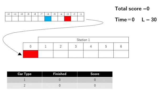
赤い矩形は車種1のベルトコンベア上での位置、青い矩形は車種2の位置を表します。
入力例 2
2 1 3 30
5
3
6
2 1
出力例 2
1
2
出力する台数が需要数より少なくても誤答とはなりません。
なお、この出力に対するスコアは 500000 です。
入力例 3
3 3 3 25
3 4 2
2 3 3
4 2 4
4 10 15
2 3 1
出力例 3
6
1 2 3 1 2 2
この出力では車種 1 を2つ、車種 2 を1つ、車種 3 を1つ、時間内に製造することができます。
このときスコアは、\mathrm{round}( {10^6\over M}(\sqrt{m_1/n_1} + \sqrt{m_2/n_2} + \sqrt{m_3/n_3}) ) = \mathrm{round}( {10^6\over 3}(1 + \sqrt{1/3} + 1) ) = 859117 となります。
Story
You are working in a car factory as part of the production control team. Plans are currently underway to build a new production line to meet increasing demand which when completed is hoped will significantly increase production capacity. However, people don't know exactly what the production capacity of the new production line will be. So being the brilliant programmer that you are, you have decided to find out how much the new production line can meet the required demands.
Problem Statement
In the production line there is a long, single link conveyer belt. The line will produce M types of cars (1, 2, \dots, M), all of which will be put on the conveyor belt and be manufactured in an assembly line. The conveyor belt is manned by S workers, who attach parts to the cars as they flow by. The cars flow at intervals of T seconds (except when the conveyor belt stops, as described below).
Each worker has a defined range of movement, and can work on cars within that range, but not on cars outside it. In order to state the conditions precisely, we will assume that the real number coordinates are set along the conveyor belt. The direction of travel of the conveyor belt is positive. To simplify the formulation, we assume that the conveyor belt extends infinitely at both ends. If the workers are assigned the numbers 1, 2, \dots, S in sequence, then worker j can only work when the coordinates of the car to be worked on fall within the closed interval [x_{j-1}+1, x_j] (where x_0 = 0 < x_1 < \dots < x_S). That is, a worker j can work on a car when its coordinates reach x_{j-1}+1, and cannot work on it when its coordinates exceed x_j. This interval is called the work station j.
It takes t_{i,j} seconds to work on a car of type i at work station j.
It is not possible for one worker to work on more than one car at the same time. If more than one car is present at a work station, the car which has the larger coordinates is worked on first.
The conveyor belt is normally moving at a speed of 1 per second, but if the work at a work station cannot be completed in time (i.e. there is an unfinished car at the end of the work station), it will stop temporarily until the work is completed. Since all the cars are on the same conveyor belt, the movement of all the cars will stop while the conveyor belt is stopped. Therefore, the longer the stoppage, the less efficient the production is, since the finished car cannot move to the next work station while the conveyor belt is stopped.
A car type i has a demand of n_i cars per day. The daily working time is limited to a maximum of L seconds. You must plan to meet the demand as much as possible within this time limit.
The plan is represented by a non-negative integer K, representing the number of cars to be made that day, and a sequence of numbers p_1, p_2, \dots, p_K of length K. The p_k is the car type of the kth car to be built. However, we assume that at most n_i cars of type i can be made.
Input
The input is given in the below format:
M S T L
t_{1, 1} ... t_{1, S}
t_{2, 1} ... t_{2, S}
:
t_{M, 1} ... t_{M, S}
x_1 x_2 ... x_S
n_1 ... n_M
Where the input values are all integers. The test cases used for the provisional tests and system tests satisfy the following conditions:
- (M, S) = (20, 40), (40, 80)
- T = 60
- 1 \le L
- 0 < t_{i,j} (1 \le i \le M, 1 \le j \le S)
- t_{i,1} < x_1, t_{i,j} < x_j - x_{j-1} (1 \le i \le M, 2 \le j \le S)
- T < x_1, T < x_j - x_{j-1} (1 \le i \le M, 2 \le j \le S)
- 1 \le n_i (1 \le i \le M)
- n_1 + n_2 + \dots + n_M = 1000
Output
Please output your result in the format below. If the ouput does not satisfy the planning requirements then it is considered a wrong answer.
K
p_1 p_2 ... p_K
Note that it is allowed that K < n_1 + n_2 + \dots + n_M. It is not a wrong answer if the number of units outputed is less than the amount demanded.
Scoring
Simulate the production line until the time limit "L" is reached or all the cars have been manufactured (see below). Assuming that all cars i are manufactured in m_i units when the simulation is finished, the score is determined as follows:
- If m_i = n_i for all i and the time at which all the cars are completed is t, then 10^6 \times (2 - {t \over L}) rounded to the nearest integer
- Otherwise, \displaystyle{{10^6 \over M}\sum_{i=1}^M \sqrt{m_i \over n_i}} rounded to the nearest integer
How to Simulate
The production line is simulated as seen below. In reality the position of the car and the progress of the work change constantly but for the sake of simplicity we are assuming that they change discretely in 1 second intervals.
We use the following variables:
- b: Flag indicating whether the conveyor belt is stationary or moving
- t: Current time
- y_k: Coordinates of the kth car to make.
- r(k, j): Progress of the work (k, j). The work (k, j) refers to the work at the work station j of the kth car.
Assignments to variables are denoted by \gets. Also, the work (k, j) is complete if and only if r(k, j) = t_{p_k, j}.
- Initialize t \gets 0 and y_k \gets -(k-1)\times T, r(k, j) \gets 0.
- Repeat the following until t = L or the work (N, S) is completed.
- If there is a pair of k, j satisfying "x_j = y_k and work (k, j) is not completed", then b \gets 1. If there is no such pair, set b \gets 0.
- For each work station j, if there is a k satisfying "the k-th car is in the work station of j and the work (k, j) is incomplete", increase r(k, j) by 1 for the smallest such k. If there is no such k, we do nothing.
- If b = 0, increase y_k by 1 for all k. If b = 1, then y_k is unchanged.
- Increase time t by 1.
- Let m_i be the number of cars of type i completed at this time. More precisely, let m_i be the number of k satisfying r(k, S) = t_{p_k,S} and p_k = i.
Input Generation
The test cases used for provisional and system tests are generated in the following way. However, some details have been omitted, so please see testcase_generator.cpp if you want to know more.
Parameters
- \alpha = 0.5, 0.7, 0.8 (the larger the value, the longer the working time t_{i,j})
- \beta = 1.0.
- c = 1.0, 1.1 (the larger the value, the longer the work station length x_j-x_{j-1}-1)
- d = 0.1.
- f = 0, 1 (When f = 1, the input contains one prototype. The worker is not familiar with the procedure for prototypes, so the operation may take longer than for other types)
- s = 3, 4 (used to determine the values of M, S etc.)
For each of the 20 possible combinations, excluding the case where \alpha = 0.8 and c = 1.0 from the 24 possible combinations, 5 cases are generated for provisional testing and 50 cases are generated for system testing.
The list of parameters used to generate the test cases for system testing (parameters_systemtest_onlinejudge.txt; md5=4a1081f7fd143943def4e95c4979b6a6) will be made available after the contest.
Overview of the generation method
Functions that randomly generate real numbers and integers between x and y (inclusive) are represented as \mathrm{rand}(x, y) and \mathrm{randint}(x, y), respectively.
- Let M = 5 \times 2^{s-1}, S = 5 \times 2^s, T = 60, N = 1000.
- Determine t_{i,j} so that it is not extremely large with respect to T. (See below for details)
- Determine a positive real number w_i. The w_i is called the production ratio of car type i. The larger \sum_j t_{i,j} is for i, the smaller w_i tends to be. (See below for details)
- Let x_1 = l_1 + 1, x_j = x_{j-1} + l_j + 1, where l_j is the length of work station j, defined as l_j = \max(T, \max_i t_{i,j} \times c).
- L = \mathrm{round}(\mathrm{rand}(1-d, 1+d) \times (T \times N+x_S)).
- If f = 1, a car of type M is a prototype. Change the working time: t_{M,j} \gets \mathrm{randint}(t_{M,j}, x_j - x_{j-1} - 1). This change is made after the determination of x_j etc. above.
- The n_i is determined by initializing n_i = 1 and repeating the following operation N-M times.
- Select one car type i which is not a prototype and increase n_i by 1. The probability that i is selected is proportional to w_i.
Outline of how t_{i,j}, w_i is determined
- Let A = P = 2^s.
- The S work stations are divided into P intervals. Each of the P intervals is called a process. The processes are numbered by 1, 2, \dots, P.
- An example of this division for the case S = 10, P = 3 is the following: process 1 consists of work stations 1, 2 and 3; process 2 consists of work stations 4, 5 and 6; process 3 consists of work stations 7, 8, 9 and 10.
- The car has several attributes. The attributes are numbered 1, 2, \dots, A. For each car type i, the set of attributes it has is determined randomly (not necessarily uniformly).
- Each attribute may affect the work of the process. For example, it may cause some processes to require additional work, such as the installation of additional parts, which increases the working time of the process. For each attribute, the process (or processes) to be affected and the degree of effect are determined randomly (not necessarily uniformly). We write X_{a,p} for the influence of attribute a on process p. The degree of influence is a non-negative real number and X_{a,p} = 0 if there is no influence.
- We define the load on process p for car type i as L_{i,p} = 1 + \sum_a X_{a,p}, where \sum_a is the sum over all the attributes a of the car type i.
- Define the production ratio for car type i as w_i = \displaystyle{\frac{\left(\sum_p L_{i,p}\right)^{-1.5}}{\sum_i \left(\sum_p L_{i,p}\right)^{-1.5}}}.
- Assign a work station to each process. The number of work stations S_p allocated to each process p should be approximately proportional to \sum_i L_{i,p}w_i.
- Let the total working time of process p be u_{i,p} = \max(S_p, \mathrm{round}(T_0 \times L_{i,p} \times \mathrm{rand}(\alpha, \beta))). The T_0 is simply a constant to ensure that the working time does not reach extreme values, and is determined so that T_0 \sum_{i,p}\frac{L_{i,p}w_i}{S_p P} = T. Starting with t_{i,j} initialized at 1, the following operations are performed u_{i,p} - S_p times.
- Choose a work station j belonging to process p uniformly at random and increase t_{i,j} by 1.
Tools
You can download the following tools here.
- visualizer.html, README-visualizer.txt
- output_checker.cpp: Program used to score the submissions.
- testcase_generator.cpp: Program used to generate input tables. Takes parameters from standard input and generates a test case.
- example-*.txt: Input and output data for practice. Please note that the data is smaller than what is actually used for judging.
- parameters_provisional.txt, parameters_systemtest.txt: This is a list of parameters for generating the equivalent test cases for provisional and system tests. The parameters are the same as for the actual test cases, except for random seeds.
testcase_generator.cpp Usage and Example
You can generate a test case yourself by compiling testcase_generator.cpp and passing in the contents of a parameter file.
For example, if you do the following in the directory where testcase_generator.cpp and parameters_provisional.txt are placed, 100 test cases will be output under provisional with the name inputXXXX.txt.
g++ -o testcase_generator testcase_generator.cpp
mkdir provisional
cd provisional
../testcase_generator < ../parameters_provisional.txt
The input part of the file name can be specified as an argument to testcase_generator.
../testcase_generator provisional < ../parameters_provisional.txt
output_checker.cpp Usage and Example
If you compile output_checker.cpp and run it with the command line arguments "input file name" and "output file name from the program of your solution" in that order, the score will be output.
g++ -o output_checker output_checker.cpp
./your_solution < provisional/input0001.txt > output0001.txt
./output_checker provisional/input0001.txt output0001.txt
Please note that the solution program uses standard input and output but the output_checker takes a filename as a command line argument.
Sample Input 1
2 1 3 30
5
3
6
2 1
Sample Output 1
3
1 1 2
In this input, there are 1 work stations, 2 car types, 5 work time for car type 1 and 3 work time for car type 2 at work station 1.
In this output, all the cars have been manufactured by the time 14 is reached.
The score is \mathrm{round}( 10^6 \times (2 - {14 \over 30}) ) = 1533333.
Please refer to the following gif for the movement on the conveyor belt.
The red rectangle represents the position of car type 1 on the conveyor belt, the blue rectangle represents the position of car type 2.
Sample Input 2
2 1 3 30
5
3
6
2 1
Sample Output 2
1
2
It is not a wrong answer if the number of units outputed is less than the amount demanded.
Furthermore, the score for this output is 500000.
Sample Input 3
3 3 3 25
3 4 2
2 3 3
4 2 4
4 10 15
2 3 1
Sample Output 3
6
1 2 3 1 2 2
With this output, we can manufacture two 1 car types, one 2 car type and one 3 car type in time.
The score is then \mathrm{round}( {10^6\over M}(\sqrt{m_1/n_1} + \sqrt{m_2/n_2} + \sqrt{m_3/n_3}) ) = \mathrm{round}( {10^6\over 3}(1 + \sqrt{1/3} + 1) ) = 859117.