Time Limit: 60 sec / Memory Limit: 1024 MiB
目次
問題概要
タイムスケジュールと空間構造
ナノグリッド
電力需給
EV
ナノグリッドの蓄電池の充放電処理
採点方法
問題文 A
入出力形式1
入出力形式2
入出力形式3
入出力制約
入出力例
サンプルコード A
問題概要
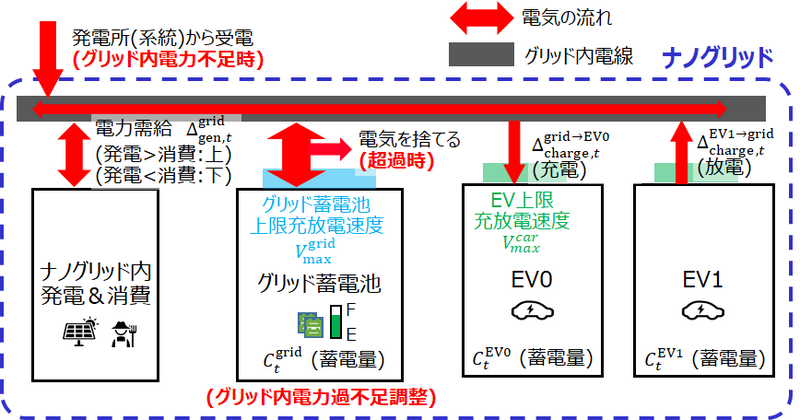
この問題では、点在するナノグリッド(発電、蓄電、消費が行われる)における電力が不足しないよう、複数台のEV(=電気自動車)を用いて蓄電量のバランスを保つことを考える。EVは走行距離に応じて電気を消費するため、ナノグリッドから充電する必要がある。ナノグリッドでは太陽光や燃料エンジンによる発電、電力の消費およびEVへの充電が行われており、それらにより時間変動する電力需給を蓄電池の充放電および必要があれば外部からの電力供給によりバランスしている。

本ページ下部からダウンロード可能なtoolkitには、ジャッジからのデータ読込などI/O周りを既に実装したサンプルコードを用意しています。また、EVの動作も"all stay", "random walk"をサンプルとして実装済です。新しいアルゴリズムを実装する際も、strategy classを継承する形でEVの動作の記述に注力できるつくりになっています(詳しくはREADME.mdもご参照ください)。投稿の際、こちらをご活用いただいて構いません。
タイムスケジュールと空間構造
- タイムスケジュール: 1つのテストケースは 1 営業日分に相当する。時刻 t は 0 から T_{\max} までの整数の値をとる。各テストケースで天候が 4 パターンのいずれかから 1 つランダムに割り当てられ、電力需給に影響を及ぼす。コンテスタントはテストケース開始時に全時刻分の予測電力需給の情報を受け取る。また各時刻 t において、各ナノグリッドの蓄電量と、前時刻 t-1 における実際の電力需給、余剰で捨てた電力、外部からの供給電力を受け取る。これらの情報を基に、コンテスタントは時刻 t から t+1 の間に実行するEVの動作(移動、充放電など) を決定する。
- 空間構造: 単純かつ無向であるグラフ G = (V, E) を考える。ここで V は頂点集合、E は辺集合である。EVの移動や充放電は全てこのグラフ内で行われる。頂点のうち一定数はナノグリッドに対応する。また、辺は道路に対応し、各辺には正の整数で重み(距離)が定められている。地図を表すグラフは、後述のアルゴリズムによってランダムに生成される。
グラフ G の生成について
全てのテストケースにおいてグラフ G = (V, E) は以下のアルゴリズムによって生成される。- 入力:|V|, |E|, \mathrm{MaxDegree}=5(最大次数)
- 頂点の生成方法:
- はじめに、|V| = R^{2} + r を満たす最大の非負整数R を見つける(ただし、r も非負整数とする)。
- 次に、0 \leq x, y < R を満たすxy座標平面上の全ての格子点に対して、点 (x, y) をプロットする。
- 各点の座標を (x, y) \leftarrow (x + dx, y + dy) とずらす。ここで dx, dy は dx, dy \in [0, 1] を満たす一様ランダムな実数である。つまり、移動後の座標は(x + dx, y + dy)\in [0,R] \times [0,R]を満たす。
- 残りの r 個の点それぞれについて、座標 (x', y') (0 \leq x', y' \leq R の一様ランダムな実数) を定めてプロットする。
- 各点に対して、1から|V|までの番号(ID)をランダムに割り振る。
- 連結性の保証:
- 生成した頂点集合 u \in V に対して、完全グラフ G_{\text{comp}} を生成する。各頂点ペア u, v \in V \times V に対する頂点間のユークリッド距離を、完全グラフにおける辺の重み W_{u, v} と定める。
- 次に、完全グラフ G_{\text{comp}} に対して、最小全域木 を生成し、生成された |V|-1 本の辺を道路とする。これらの辺の重み d_{u,v} を d_{u,v} \leftarrow \lceil 2 \times W_{u, v} \rceil と定める。
- 残りの道路の作成方法:
- 残りの |E|-(|V|-1) 本の道路は、次の手順で1本ずつ生成される。
- \mathrm{cost}(u,v)を更新する。
- グラフGの辺でつながっていないu, vのペアの内、\mathrm{cost(u,v)}の最小を与えるペアをつなぐ辺\left\{ u, v \right\}をグラフGに加える。
- 選ばれた辺の重み d_{u,v} を d_{u,v} \leftarrow \lceil 2 \times W_{u, v} \rceil と定める。
-
ここで \mathrm{cost}(u,v) のベースは頂点間のユークリッド距離だが、低い次数の頂点が選ばれやすくなるように、また、できる限り道の交差を避けるため、斜め方向よりも縦横方向の道が選ばれやすくなるように \mathrm{cost}(u,v) を定める。以下に \mathrm{cost}(u,v) の計算方法の詳細を示す。
- 各頂点 u\in V の次数 \mathrm{degree}(u) を計算する。次数 \mathrm{degree}(u) は u\in V をいずれかの端点に含むグラフ G の辺の本数である。
- 各頂点 u\in V の色を、頂点の初めの(ずらす前の)座標 (x,y) をもとに、下記のように定める。まずは |V| 個の頂点のうち、R^{2} 個の頂点に対し、
- x+y が偶数の場合 : \mathrm{color}(u) = 0
- x+y が奇数の場合 : \mathrm{color}(u) = 1
- と定める。残りの r 個の頂点には、ランダムに0もしくは1の色を割り当てる。
- ファクター f(u,v) を以下のように定める:
- \mathrm{color}(u) と \mathrm{color}(v) が同じ場合: \mathrm{f}(u,v) = 5
- \mathrm{color}(u) と \mathrm{color}(v) が異なる場合: \mathrm{f}(u,v) = 1
- ファクター g(u) を以下のように定める:
- \mathrm{degree}(u) \lt \mathrm{MaxDegree} の場合: g(u)=1
- \mathrm{degree}(u) \geq \mathrm{MaxDegree} の場合: g(u)=\infty
- \mathrm{cost}(u,v) を以下のように計算する。:
- \mathrm{cost}(u,v) = W_{u,v}\times \mathrm{degree}(u) \times \mathrm{degree}(v) \times f(u,v) \times g(u) \times g(v).
- 残りの |E|-(|V|-1) 本の道路は、次の手順で1本ずつ生成される。
- ナノグリッド頂点の選択方法:
- 頂点集合 u \in V の中から一様ランダムに N_{\mathrm{grid}} 個の頂点を選択し、それらをナノグリッド頂点と定める。またナノグリッド頂点集合を V_{\mathrm{grid}} と表す。
ナノグリッド
ナノグリッドは発電設備、電力消費者、EVの充放電設備および蓄電池から構成され、以下の内部状態を持つ。
-
頂点ID: 頂点 u のID. ただし、u \in V_{\mathrm{grid}} (V_{\mathrm{grid}}: ナノグリッド頂点集合, ("グラフG の生成について"を参照))
-
蓄電量: ナノグリッド内の蓄電池に蓄えられた電気の量。初期値 C_{\mathrm{init}}^{\mathrm{grid}}。上限値 C_{\mathrm{max}}^{\mathrm{grid}} (初期値と上限値は全ナノグリッド共通)。各時刻 t で電力需給(=発電-消費)の値だけ増減する。また、EVと蓄電池の間の充放電によっても増減する(詳細は ナノグリッドの蓄電池の充放電処理 参照)。増加分が上限値 C_{\mathrm{max}}^{\mathrm{grid}} を超える場合、次の時刻 t+1 の蓄電量は上限値となり、超えた分の電気は捨てられる。逆に蓄電量が足りなくなった場合、不足分はナノグリッドの外部(系統電力)から供給され、不足分に比例してスコアは減点される(詳細は採点方法参照)。
-
電力需給: 各時刻におけるナノグリッド内の発電量とEVへの充電及び蓄電池への蓄電量を除いた消費量の差であり、その各時刻における予測値が時系列データで各テストケース開始時にコンテスタントに与えられる。実際の電力状態はその予測値と確率的部分(ゆらぎ、ゲリラ豪雨or想定外の晴れ)の和になる(詳細は電力需給参照)。
-
上限充放電速度: V_{\max}^{\mathrm{grid}}. ナノグリッド内の蓄電池への充放電速度の上限値(全ナノグリッド共通)
電力需給
各時刻におけるナノグリッド内の発電量とEVへの充電及び蓄電池への蓄電量を除いた消費量の差である。
-
電力需給のパターン: 1つのテストケースは 1 営業日分(0 \leq t < T_{\max})に対応する。テストケース開始時に、その日の天候が晴(ゲリラ豪雨無し)、晴(ゲリラ豪雨有り)、雨(想定外の晴れ無し)、雨(想定外の晴れ有り)の 4 種類から選ばれ、コンテスタントに通知される。天候によってナノグリッド内の発電量(太陽光発電)が変化するため、予測電力需給の 1 営業日分の総和は晴れ(ゲリラ豪雨無し)の場合が最も多く、逆に雨(想定外の晴れ無し)の場合は最も少なくなる。各ナノグリッドには需要パターンの異なる N_{\mathrm{pattern}} 種類の予測電力需給パターンから 1 つがランダムに割り当てられ、どのパターンが割り当てられたかはコンテスタントに通知される。また、予測電力需給の各時刻の値は、テストケース開始時にコンテスタントに通知される。
-
電力需給の値: 電力需給の値は予測電力需給と確率的な揺らぎ \delta とゲリラ豪雨及び想定外の晴れによる変化量の和で表される。
- 予想電力需給: 時間 0 \leq t < T_{\max} を N_{\mathrm{div}} 等分の区間に分け、同一区間内で予測電力需給は一定とする。
- 確率的揺らぎ: 各時刻 t で予測電力需給に確率的な揺らぎ値 \delta が加わる。\delta は各時刻、各ナノグリッド独立に平均 0、分散 \sigma^{2}_{\mathrm{ele}} の正規分布から生成され、その値はコンテスタントには事前に通知されない。
- ゲリラ豪雨: 天候が"晴(ゲリラ豪雨有り)"の場合、N_{\mathrm{div}} つの各時間区間において p_{\mathrm{event}} の確率でゲリラ豪雨が発生する。確率は時間区間ごと独立かつ一定である。ゲリラ豪雨が発生すると、その時間区間内の全時刻 t で、時間区間ごと独立且つランダムに選ばれた 15\%(端数切捨て)のナノグリッドの電力需給が \Delta_{\mathrm{event}} だけ減少する(太陽光による発電量が想定よりも大幅に減少する)。
- 想定外の晴れ: 天候が"雨(想定外の晴れ有り)"の場合、ゲリラ豪雨と同じ確率で想定外の晴れが発生する。想定外の晴れが発生すると、その時間区間内の全時刻 t で、時間区間ごと独立且つランダムに選ばれた 15\%(端数切捨て)のナノグリッドの電力需給が \Delta_{\mathrm{event}} だけ増加する(太陽光による発電量が想定よりも大幅に増加する)。
ゲリラ豪雨及び想定外の晴れの発生タイミングは事前にコンテスタントには通知されない。最終的な電力需給の値は、予測電力需給 + \delta \pm \Delta_{\mathrm{event}} となる。

EV
コンテスタントは複数台のEVを操作し、ナノグリッド間の電力バランス調整を行う。
-
台数: EVの台数は、テストケースの開始時に区間 [N_{\min}^{\mathrm{EV}}, N_{\max}^{\mathrm{EV}}] から一様ランダムに選ばれ、コンテスタントに通知される。
-
初期位置: テストケース開始時にナノグリッド含む全ての頂点からEV台数に等しい数の頂点をランダムに選び、EVは選ばれた各頂点に 1 台ずつ配置される。
-
内部状態: 各EVは以下の内部状態を持つ
- ID (0, 1,... , N^{\mathrm{EV}}-1)
- 蓄電量 C^{\mathrm{EV}}_{t} (非負整数, 初期値は C^{\mathrm{EV}}_{t=0}、上限値は C^{\mathrm{EV}}_{\max} で共に全EV共通)
- 位置 (頂点上もしくは辺上)
- 上限充放電速度 V_{\max}^{\mathrm{EV}} (EVの充放電速度の上限値 (全EV共通))
-
動作: コンテスタントは各時刻 t における各EVの動作を以下から選び、決定する。
stay: 移動せずその場にとどまる。この場合、EVの蓄電量は消費されない。(C^{\mathrm{EV}}_{t+1}-C^{\mathrm{EV}}_{t}=0)-
move w: 頂点 w \in V の方向に向かって距離 1 だけ進む。次の時刻のEVの蓄電量は \Delta^{\mathrm{EV}}_{\mathrm{move}} だけ減少する。ただし、以下の条件を満たしており、且つ移動後のEVの蓄電量が負になる場合(C^{\mathrm{EV}}_{t} - \Delta^{\mathrm{EV}}_{\mathrm{move}} < 0)、EVの蓄電量は減らず、stayが実行された場合と同じ挙動となる(その場に留まる)。move wを選択するとき、w が以下の条件を満たさない場合、WA(Wrong Answer) となる。- w は w \in V を満たす頂点である
- EVが頂点 u \in V 上にいる場合、頂点対 \left\{ u, w \right\} がグラフの辺集合に含まれていなければならない。すなわち、\left\{ u, w \right\} \in E でなければならない
- EVが辺 \left\{ u, v \right\} 上にいる場合、w = u または w = v でなければならない
-
charge_from_grid\Delta^{\mathrm{grid} \rightarrow \mathrm{EV}}_{\mathrm{charge}}: ナノグリッド上でEVへ \Delta^{\mathrm{grid} \rightarrow \mathrm{EV}}_{\mathrm{charge}} だけ充電する。そのとき次の時刻 t+1 でのEVの蓄電量 C^{\mathrm{EV}}_{t+1} は、C^{\mathrm{EV}}_{t+1} \leftarrow C^{\mathrm{EV}}_{t} + \Delta^{\mathrm{grid} \rightarrow \mathrm{EV}}_{\mathrm{charge}} となる。同一ナノグリッドから複数台のEVに同時に充電することも可能である。また、同一ナノグリッド上で同時に別のEVからナノグリッドへ放電charge_to_gridすることも可能である(動作は後述)。charge_from_grid\Delta^{\mathrm{grid} \rightarrow \mathrm{EV}}_{\mathrm{charge}} を選択するとき、以下の条件を満たさない場合、WA(Wrong Answer) となる。- EVはナノグリッドの頂点 u \in V_{\mathrm{grid}} に居る
- \Delta^{\mathrm{grid} \rightarrow \mathrm{EV}}_{\mathrm{charge}}は自然数である。
- EVの上限充放電速度を超えない: \Delta^{\mathrm{grid} \rightarrow \mathrm{EV}}_{\mathrm{charge}} \leq V_{\max}^{\mathrm{EV}}
- 充電後のEVの蓄電量が上限を超えない: C^{\mathrm{EV}}_{t} + \Delta^{\mathrm{grid} \rightarrow \mathrm{EV}}_{\mathrm{charge}} \leq C^{\mathrm{EV}}_{\max}
-
charge_to_grid\Delta^{\mathrm{EV} \rightarrow \mathrm{grid}}_{\mathrm{charge}}: EVからナノグリッドへ \Delta^{\mathrm{EV} \rightarrow \mathrm{grid}}_{\mathrm{charge}} だけ放電する。そのとき次の時刻 t+1 でのEVの蓄電量 C^{\mathrm{EV}}_{t+1} は、C^{\mathrm{EV}}_{t+1} \leftarrow C^{\mathrm{EV}}_{t} - \Delta^{\mathrm{EV} \rightarrow \mathrm{grid}}_{\mathrm{charge}} となる。同一ナノグリッドへ複数台のEVから同時に放電することも可能である。また、同時に同一ナノグリッド上で別のEVへ充電charge_from_gridすることも可能である。charge_to_grid\Delta^{\mathrm{EV} \rightarrow \mathrm{grid}}_{\mathrm{charge}} を選択するとき、以下の条件を満たさない場合、WA(Wrong Answer) となる。- EVはナノグリッドの頂点 u \in V_{\mathrm{grid}} に居る
- \Delta^{\mathrm{EV} \rightarrow \mathrm{grid}}_{\mathrm{charge}}は自然数である。
- EVの上限充放電速度を超えない: \Delta^{\mathrm{EV} \rightarrow \mathrm{grid}}_{\mathrm{charge}} \leq V_{\max}^{\mathrm{EV}}
- 放電後のEVの蓄電量が負にならない: C^{\mathrm{EV}}_{t} - \Delta^{\mathrm{EV} \rightarrow \mathrm{grid}}_{\mathrm{charge}} \geq 0
ナノグリッドの蓄電池の充放電処理
各ナノグリッドにおいて、発電量、消費量及び接続したEVの充放電によって時々刻々とナノグリッドの蓄電量は増減する。本処理により、各時刻各ナノグリッド内の電力需給(=発電量-消費量)とEVの充放電量を足し合わせ、余剰があればナノグリッド内の蓄電池に充電し、逆に足りなければ蓄電池から放電する。余剰が多い場合、蓄電池の上限充電速度を超える分、もしくは上限蓄電容量を超える分の電気は捨て、不足電力が多い場合、蓄電池の上限放電速度を超える分、もしくは蓄電量が枯渇しても足りない分の電気は、ナノグリッド外(系統)から購入する。いずれの場合も、コンテスタントが指定したEVの充放電量の分だけ、次の時刻で必ず充放電される。
具体的には、各時刻 t において、次の時刻 t+1 の各ナノグリッドの蓄電量を決定するため、以下の処理1~4が実行される。
-
処理1: ナノグリッド内の時刻 t における電力収支 \Delta^{\mathrm{grid}}_{\mathrm{total}} を計算する
\Delta^{\mathrm{grid}}_{\mathrm{total}} = \Delta^{\mathrm{grid}}_{\mathrm{gen},t} - \sum_{i \in \mathrm{all EV}} \Delta^{\mathrm{grid} \rightarrow \mathrm{EV}i}_{\mathrm{charge},t} + \sum_{i \in \mathrm{all EV}} \Delta^{\mathrm{EV}i \rightarrow \mathrm{grid}}_{\mathrm{charge},t}
ここで、各変数は以下の通りである。- \Delta^{\mathrm{grid}}_{\mathrm{gen},t}: 時刻 t における電力需給であり、予測電力需給 \Delta^{\mathrm{grid,predict}}_{\mathrm{gen},t} と 確率的部分(ゆらぎ、ゲリラ豪雨or想定外の晴れ)の和である。ここで、予測電力需給の値はテストケースの開始時にコンテスタントに通知されるが、確率的部分は時刻 t ではコンテスタントに通知されないことに注意せよ(ただし次の時刻 t+1 で \Delta^{\mathrm{grid}}_{\mathrm{gen},t} がコンテスタントに通知される(詳しくは"入出力形式2"を参照))。
- \Delta^{\mathrm{grid} \rightarrow \mathrm{EV}i}_{\mathrm{charge},t}: ナノグリッドからEViへの充電量であり、コンテスタントが時刻 t で指定する。
- \Delta^{\mathrm{EV}i \rightarrow \mathrm{grid}}_{\mathrm{charge},t}: EViからナノグリッドへの放電量であり、コンテスタントが時刻 t で指定する。
-
処理2: 電力収支が大きい、つまり余剰電力が大きい場合の処理。
\Delta^{\mathrm{grid}}_{\mathrm{total}} \geq \min \left\{ V_{\max}^{\mathrm{grid}}, C^{\mathrm{grid}}_{\max}-C^{\mathrm{grid}}_{t} \right\} の場合、次の時刻 t+1 のナノグリッドの蓄電量を以下のように定める。
C^{\mathrm{grid}}_{t+1} \leftarrow C^{\mathrm{grid}}_{t}+\min \left\{ V_{\max}^{\mathrm{grid}}, C^{\mathrm{grid}}_{\max}-C^{\mathrm{grid}}_{t} \right\}
つまり、速度や上限蓄電量を超えた分の電気は蓄電池に充電されない(捨てられることになる)。 -
処理3: 電力収支が小さい、つまり不足電力が大きい場合の処理。
\Delta^{\mathrm{grid}}_{\mathrm{total}} < - \min \left\{ V_{\max}^{\mathrm{grid}}, C^{\mathrm{grid}}_{t} \right\} の場合、次の時刻 t+1 のナノグリッドの蓄電量を以下のように定める。
C^{\mathrm{grid}}_{t+1} \leftarrow C^{\mathrm{grid}}_{t} - \min \left\{ V_{\max}^{\mathrm{grid}}, C^{\mathrm{grid}}_{t} \right\}
また、上記では、ナノグリッド内の電力不足分:
- \Delta^{\mathrm{grid}}_{\mathrm{total}} - \min \left\{ V_{\max}^{\mathrm{grid}}, C^{\mathrm{grid}}_{t} \right\}(>0)
をナノグリッド外(系統電力など)から購入する。そのため、不足分に比例してスコアが減点される(詳細は採点方法参照)。 -
処理4: 電力収支が適度な大きさの場合の処理。
処理2及び処理3が共に実行されない場合、電力収支の分だけ次の時刻 t+1 のナノグリッドの蓄電量を増減させる。
C^{\mathrm{grid}}_{t+1} \leftarrow C^{\mathrm{grid}}_{t} + \Delta^{\mathrm{grid}}_{\mathrm{total}}
採点方法
-
コンテスト開催中の順位は 16 つのテストケースのスコアの合計値で決定する。16 つのテストケースのうち、晴(ゲリラ豪雨無し)、晴(ゲリラ豪雨有り)、雨(想定外の晴れ無し)、雨(想定外の晴れ有り)の数はそれぞれ 6, 2, 6, 2 で固定である。
-
各テストケースにおいて以下のようにスコアを計算する。
\mathrm{Score}=\sum_{i=1}^{N_{\mathrm{EV}}} C_{t=T_{\max}}^{\mathrm{EV}i} + \sum_{i=1}^{N_{\mathrm{grid}}} C_{t=T_{\max}}^{\mathrm{grid}i} - \gamma \sum_{t=0}^{T_{\max}-1} \sum_{i=1}^{N_{\mathrm{grid}}} L_{i,t} + 3000000
ただし、第 1 項と第 2 項は t=T_{\max} 時点での全EV及び全ナノグリッドの残り蓄電量であり、\gamma は不足電力ペナルティ係数、L_{i,t} は時刻 t のナノグリッド i における不足電力であり、ナノグリッドの蓄電池の充放電処理の処理3が実行された場合 L_{i,t} = - \Delta^{\mathrm{grid}}_{\mathrm{total}} - \min \left\{ V_{\max}^{\mathrm{grid}}, C^{\mathrm{grid}}_{t} \right\}(L_{i,t}>0) であり、処理3が実行されない場合は L_{i,t}=0 である。 -
システムテストは、ツールキットで開示済の 6(=N_\mathrm{pattern} \times 2(晴,雨)) パターンの予測電力需給パターンを用いた 160 個のテストケースに加えて、未開示の 6(=N_\mathrm{pattern} \times 2(晴,雨)) パターンの予測電力需給パターンを用いた 40 個のテストケースから成る、計 200 個のテストケースで実施します。なお、ゆらぎの平均・分散値や、ゲリラ豪雨及び想定外の晴れによる電力需給の変動幅、発生確率及び発生条件は同じです。
詳細な内訳は下記表をご覧ください*
| 予測電力需給(開示済) | 予測電力需給(未開示) | 合計 | |
|---|---|---|---|
| 晴(ゲリラ豪雨無) | 60 | 15 | 75 |
| 晴(ゲリラ豪雨有) | 20 | 5 | 25 |
| 雨(想定外の晴無) | 60 | 15 | 75 |
| 雨(想定外の晴有) | 20 | 5 | 25 |
| 合計 | 160 | 40 | 200 |
* 12/18にyuusanlondon様から頂いたご質問に対する回答から、システムテストの内容に一部変更が入ってしまい大変申し訳ありません。運営側で検討させて頂いた結果、上記の内容で最終順位を決定させて頂きたく、ご理解頂けますと幸いです。
(12/29追記) 未開示の予測電力需給パターンの生成法やジェネレーターを開示する予定はございません。
ただし、未開示のパターンでの電力スコアの満点(理想的な制御実行時の得点の上限)は、開示済のパターンの電力スコアの満点と同等の得点となるよう、作成予定です。
問題文 A
問題 A はインタラクティブな問題である。 得点(Score)を最大化するように電力をマネジメントするアルゴリズムを作ることが問題 A のタスクである。 Contestantが高得点を獲得するためには、確率的に上下する電力需給に対して、蓄電池を持ちグラフ上を移動する電気自動車(EV)とナノグリッドとの間で必要に応じて充放電を行い、蓄電池を有するナノグリッドの蓄電量を管理することが必要となる。 作成するプログラムの得点判定の際は、コンテスタント側とジャッジ側が以下で示す流れに沿って処理を行う。
| 繰り返し処理 | コンテスタント | ジャッジ |
|---|---|---|
| グラフ G を出力 | ||
| 電力需給の情報を出力 | ||
| ナノグリッドの情報を出力 | ||
| EVの情報を出力 | ||
| スコアの情報を出力 | ||
| 繰り返し処理(ターン)の回数 T_\mathrm{max} を出力 | ||
| for t=0,...,T_\mathrm{max}-1 do | - | - |
| 時刻 t におけるEVとナノグリッドの状態 \mathrm{info}_t を出力 | ||
| 各EVに対して制御コマンドを出力 | ||
| end for | ||
| 時刻 t=T_\mathrm{max} におけるEVとナノグリッドの状態 \mathrm{info}_t を出力 | ||
| スコア \mathrm{Score} を出力 |
ジャッジによるグラフ、電力需給、ナノグリッド、EV、スコア、ターン数に関する情報は、はじめに1回だけ出力される。各試行で 0 \leq t \lt T_\mathrm{max} を満たす整数 t において、表で示した順番通りに毎回行われる。なお、時刻 t=T_\mathrm{max} における \mathrm{info}_t 及びスコアは必ずコンテスタント側で読み出す必要がある(読み出さない場合TLEになる可能性がある)。
入出力形式1
はじめに、グラフ G、電力需給の情報、ナノグリッドの情報、EVの情報、スコアの情報およびターン数が、以下の形式によりジャッジから標準入力に与えられる。
|V| |E|
u_1 v_1 d_1
:
u_{|E|} v_{|E|} d_{|E|}
\mathrm{DayType}
N_\mathrm{div} N_\mathrm{pattern} \sigma^{2}_{\mathrm{ele}} p_{\mathrm{event}} \Delta_{\mathrm{event}}
\mathrm{pw}_{1,1}^{\mathrm{predict}} \mathrm{pw}_{1,2}^{\mathrm{predict}} ... \mathrm{pw}_{1,N_\mathrm{div}}^{\mathrm{predict}}
:
\mathrm{pw}_{N_\mathrm{pattern},1}^{\mathrm{predict}} \mathrm{pw}_{N_\mathrm{pattern},2}^{\mathrm{predict}} ... \mathrm{pw}_{N_\mathrm{pattern},N_\mathrm{div}}^{\mathrm{predict}}
N_\mathrm{grid} C_{\mathrm{init}}^{\mathrm{grid}} C_{\mathrm{max}}^{\mathrm{grid}} V_{\max}^{\mathrm{grid}}
x_1 \mathrm{pattern}_1
:
x_{N_\mathrm{grid}} \mathrm{pattern}_{N_\mathrm{grid}}
N_\mathrm{EV} C_{\mathrm{init}}^{\mathrm{EV}} C_{\mathrm{max}}^{\mathrm{EV}} V_{\max}^{\mathrm{EV}} \Delta_{\mathrm{move}}^{\mathrm{EV}}
\mathrm{pos}_1
:
\mathrm{pos}_{N_\mathrm{EV}}
\gamma
T_\mathrm{max}
- 1 行目の |V| はグラフの頂点数、|E| はグラフの辺数である。
- 続く |E| 行で、グラフの辺が与えられる。 |E| 行のうち i 行目は、頂点 u_{i} と v_{i} の間に距離 d_i の辺が存在することを表す。
- 続く 1 行で、天候タイプ \mathrm{DayType} が与えられる。\mathrm{DayType} は 0: 晴(ゲリラ豪雨無し)、1: 晴(ゲリラ豪雨有り)、2: 雨(想定外の晴れ無し)、3: 雨(想定外の晴れ有り)のいずれかが与えられる。
- 続く 1 行で、予測電力需給が一定値となる区間の数 N_\mathrm{div} と予測電力需給のパターン数 N_\mathrm{pattern} と電力需給の分散 \sigma^{2}_{\mathrm{ele}} とゲリラ豪雨もしくは想定外の晴れの発生確率 p_{\mathrm{event}} (天候タイプが 0 もしくは 2 の場合は 0.0 となる)とゲリラ豪雨もしくは想定外の晴れ発生時の電力需給の変化量 \Delta_{\mathrm{event}} が与えられる。
- 続く N_\mathrm{pattern} 行で各パターンの予測電力需給の値が与えられる。i 行目の j 番目の数値 \mathrm{pw}_{i,j}^{\mathrm{predict}} は、予測電力需給パターン i における時間区間 j 番目の予測電力需給の値を表す。
- 続く 1 行で、ナノグリッドの個数 N_\mathrm{grid} とナノグリッドの時刻 0 での蓄電量 C_{\mathrm{init}}^{\mathrm{grid}} と最大蓄電量 C_{\mathrm{max}}^{\mathrm{grid}} と蓄電池の上限充放電速度 V_{\max}^{\mathrm{grid}} が与えられる。
- 続く N_\mathrm{grid} 行でナノグリッドの情報が与えられる。N_\mathrm{grid} 行のうち i 行目は、頂点 x_i 上に、予測電力需給パターン \mathrm{pattern}_i のナノグリッドが存在することを表す。
- 続く 1 行で、EVの個数 N_\mathrm{EV} とEVの時刻 0 での蓄電量 C_{\mathrm{init}}^{\mathrm{EV}} と最大蓄電量 C_{\mathrm{max}}^{\mathrm{EV}} と蓄電池の上限充放電速度 V_{\max}^{\mathrm{EV}} と単位距離の移動に必要な電力 \Delta_{\mathrm{move}}^{\mathrm{EV}} が与えられる。
- 続く N_\mathrm{EV} 行で、EVの位置が与えられる。N_\mathrm{EV} 行のうち i 行目は、i 番目のEVが頂点 \mathrm{pos}_i 上にあることを表す。
- 続く 1 行で、不足電力ペナルティ係数 \gamma が与えられる。
- 続く 1 行で、あなたが行動するターン数 T_{\max} が与えられる。
入出力形式2
各時刻 t に、その時刻におけるEVとナノグリッドの状態 \mathrm{info}_t が、以下の形式によりジャッジから標準入力に与えられる。
x_1 y_1 \mathrm{pw}_{1}^{\mathrm{actual},t-1} \mathrm{pw}_{1}^{\mathrm{excess},t-1} \mathrm{pw}_{1}^{\mathrm{buy},t-1}
:
x_{N_\mathrm{grid}} y_{N_\mathrm{grid}} \mathrm{pw}_{N_\mathrm{grid}}^{\mathrm{actual},t-1} \mathrm{pw}_{N_\mathrm{grid}}^{\mathrm{excess},t-1} \mathrm{pw}_{N_\mathrm{grid}}^{\mathrm{buy},t-1}
\mathrm{carinfo}_1
:
\mathrm{carinfo}_{N_\mathrm{EV}}
- 始めの N_\mathrm{grid} 行のうち i 行目は、x_i 上に存在するナノグリッドの蓄電量が y_i であり、前時刻 t-1 における実際の電力需給、余って捨てられた電気の量、電力不足で系統から購入した電気の量がそれぞれ \mathrm{pw}_{i}^{\mathrm{actual},t-1}、\mathrm{pw}_{i}^{\mathrm{excess},t-1}、\mathrm{pw}_{i}^{\mathrm{buy},t-1} であることを表す。ただし t=0 においては、 \mathrm{pw}_{i}^{\mathrm{actual},t-1}、\mathrm{pw}_{i}^{\mathrm{excess},t-1}、\mathrm{pw}_{i}^{\mathrm{buy},t-1} はいずれも 0 が表示されるものとする。
補足: \mathrm{pw}_{i}^{\mathrm{actual},t-1}、\mathrm{pw}_{i}^{\mathrm{excess},t-1}、\mathrm{pw}_{i}^{\mathrm{buy},t-1}は、それぞれ ナノグリッドの蓄電池の充放電処理 "処理1"の \Delta^{\mathrm{grid}}_{\mathrm{gen},t-1}、"処理2"の"速度や上限蓄電量を超えた分の電気"\Delta^{\mathrm{grid}}_{\mathrm{total},t-1} - \min \left\{ V_{\max}^{\mathrm{grid}}, C^{\mathrm{grid}}_{\max}-C^{\mathrm{grid}}_{t-1} \right\}、"処理3"の"電力不足分" - \Delta^{\mathrm{grid}}_{\mathrm{total},t-1} - \min \left\{ V_{\max}^{\mathrm{grid}}, C^{\mathrm{grid}}_{t-1} \right\} に対応する。ただし、前時刻 t-1 でそれぞれ"処理2"、"処理3"が実行されなかった場合、\mathrm{pw}_{i}^{\mathrm{excess},t-1} と \mathrm{pw}_{i}^{\mathrm{buy},t-1} はそれぞれ 0 となる。 - 続く N_\mathrm{EV} 項目はそれぞれ 3 行からなり、そのうち i 項目目の \mathrm{carinfo}_i は i 番目のEVの状態を表す。\mathrm{carinfo}_i はそれぞれ後述の形式で与えられる。
i 番目のEVの状態を表す \mathrm{carinfo}_i は、以下の形式で与えられる。
\mathrm{charge}_i
u_i v_i \mathrm{dist\_from}\_u_i \mathrm{dist\_to}\_v_i
N_{\mathrm{adj},i} a_{i,1} a_{i,2} \ldots a_{i,N_\mathrm{adj}}
- 始めの 1 行目は、 i 番目のEVの蓄電量が \mathrm{charge}_i であることを表す。
- 続く 2 行目は、 i 番目のEVの位置を表す。u_i \ne v_i ならば、i 番目のEVは頂点 u_i と 頂点v_i を結ぶ辺上に存在して頂点 u_i から \mathrm{dist\_from}\_u_i、頂点 v_i から \mathrm{dist\_to}\_v_i の距離にあることを表す。u_i = v_i ならば、i 番目のEVはちょうど頂点 u_i 上にあることを表し、\mathrm{dist\_from}\_u_i と \mathrm{dist\_to}\_v_i は共に 0 が出力される。
- 続く 3 行目は、動作
moveで i 番目のEVがその方向に移動可能な頂点が N_{\mathrm{adj},i} 個存在し、それらが頂点 a_{i,1}、頂点 a_{i,2}、\ldots、頂点 a_{i,N_\mathrm{adj}} であることを表す。
次に、コンテスタントは、時刻 t (0 \leq t \lt T_{\max}) における各EVの動作 \mathrm{command}_i (1 \leq i \leq N_\mathrm{EV}) を標準出力に出力しなければならない。各動作は改行で区切られなくてはならず、また末尾に改行を出力する必要がある。
\mathrm{command}_{1}
\mathrm{command}_{2}
:
\mathrm{command}_{N_\mathrm{EV}}
ここで、\mathrm{command} は以下の形式でなければならない。
stayを行う場合、stayと 1 行で出力move wを行う場合、move wと 1 行で出力charge_from_grid\Delta^{\mathrm{grid} \rightarrow \mathrm{EV}}_{\mathrm{charge}} を行う場合、charge_from_grid\Delta^{\mathrm{grid} \rightarrow \mathrm{EV}}_{\mathrm{charge}} と 1 行で出力charge_to_grid\Delta^{\mathrm{EV} \rightarrow \mathrm{grid}}_{\mathrm{charge}} を行う場合、charge_to_grid\Delta^{\mathrm{EV} \rightarrow \mathrm{grid}}_{\mathrm{charge}} と 1 行で出力
それぞれの動作には満たすべき条件が存在する(詳細はEVの"動作"の節を参照のこと)。それらの条件を満たさない場合の動作は未定義である。
入出力形式3
コンテスタントが時刻 t=T_\mathrm{max}-1 における各EVの動作を標準出力に出力したのち、ジャッジから時刻 t=T_\mathrm{max} におけるEVとナノグリッドの状態 \mathrm{info}_t が標準入力に与えられる(\mathrm{info}_t の形式は"入出力形式2"を参照)。引き続いて次の行にジャッジから以下の形式でスコア \mathrm{Score} が標準入力に与えられる。
\mathrm{Score}
入出力制約
- 入力で与えられる数値のうち"[小数]"と記載されているものは小数で与えられ、その他のものは整数で与えられる。
初期化(入出力形式1)
- |V| = 225
- 1.5 |V| \leq |E| \leq 2 |V|
- 1 \leq u_{i}, v_{i} \leq |V|, u_i \ne v_i (1 \leq i \leq |E|)
- 1 \leq d_i \leq \lceil 2\sqrt{2|V|} \rceil (1 \leq i \leq |E|)
- 与えられるグラフは自己ループ・多重辺が存在せず、連結であることが保証される。
- \mathrm{DayType} \in \left\{ 0, 1, 2, 3 \right\}
- N_\mathrm{div} = 20
- N_\mathrm{pattern} = 3
- \sigma^{2}_{\mathrm{ele}} = 100
- p_{\mathrm{event}} \in \left\{ 0.0, 0.1 \right\} "[小数]"
- \Delta_{\mathrm{event}} = 1000
- -1000 \lt \mathrm{pw}_{i,j}^{\mathrm{predict}} \lt 1000 (1 \leq i \leq N_\mathrm{pattern}, 1 \leq j \leq N_\mathrm{div})
- N_\mathrm{grid} = 20
- C_{\mathrm{init}}^{\mathrm{grid}} = 25000
- C_{\mathrm{max}}^{\mathrm{grid}} = 50000
- V_{\max}^{\mathrm{grid}} = 800
- 1 \leq x_i \leq |V| (i \neq j なら x_i \neq x_j, 1 \leq i \leq N_\mathrm{grid})
- 1 \leq \mathrm{pattern}_i \leq N_\mathrm{pattern} (1 \leq i \leq N_\mathrm{grid})
- N_{\min}^{\mathrm{EV}} = 15
- N_{\max}^{\mathrm{EV}} = 25
- N_{\min}^{\mathrm{EV}} \leq N_\mathrm{EV} \leq N_{\max}^{\mathrm{EV}}
- C_{\mathrm{init}}^{\mathrm{EV}} = 12500
- C_{\mathrm{max}}^{\mathrm{EV}} = 25000
- V_{\max}^{\mathrm{EV}} = 400
- \Delta_{\mathrm{move}}^{\mathrm{EV}} = 50
- 1 \leq \mathrm{pos}_i \leq |V| (1 \leq i \leq N_\mathrm{EV})
- \gamma = 2.0 "[小数]"
- T_\mathrm{max} = 1000
繰り返し処理(入出力形式2)
- 1 \leq x_i \leq |V| (i \neq j なら x_i \neq x_j, 1 \leq i \leq N_\mathrm{grid})
- 0 \leq y_i \leq C_{\mathrm{max}}^{\mathrm{grid}} (1 \leq i \leq N_\mathrm{grid})
- -10000 \lt \mathrm{pw}_{i}^{\mathrm{actual},j} \lt 10000 (1 \leq i \leq N_\mathrm{grid}, -1 \leq j \leq T_\mathrm{max}-2)
- 0 \leq \mathrm{pw}_{i}^{\mathrm{excess},j} \lt 10000, (1 \leq i \leq N_\mathrm{grid}, -1 \leq j \leq T_\mathrm{max}-2)
- 0 \leq \mathrm{pw}_{i}^{\mathrm{buy},j} \lt 10000, (1 \leq i \leq N_\mathrm{grid}, -1 \leq j \leq T_\mathrm{max}-2)
- 0 \leq \mathrm{charge}_i \leq C_{\mathrm{max}}^{\mathrm{EV}} (1 \leq i \leq N_\mathrm{EV})
- 1 \leq u_i, v_i \leq |V| (1 \leq i \leq N_\mathrm{EV})
- 0 \leq \mathrm{dist\_from}\_u_i \leq \lceil 2\sqrt{2|V|} \rceil (1 \leq i \leq N_\mathrm{EV})
- 0 \leq \mathrm{dist\_to}\_v_i \leq \lceil 2\sqrt{2|V|} \rceil (1 \leq i \leq N_\mathrm{EV})
- 1 \leq N_{\mathrm{adj},i} \leq 5(\mathrm{MaxDegree}) (1 \leq i \leq N_\mathrm{EV})
- 1 \leq a_{i,j} \leq |V| (1 \leq i \leq N_\mathrm{EV}, 1 \leq j \leq N_{\mathrm{adj},i})
スコア(入出力形式3)
- \mathrm{Score} "[小数]"
入出力例
注意: この例はわかりやすさのために小さなセットで入出力を説明したものである。そのためパラメータの値は"入出力制約"に書かれた値とは異なるが、入出力のフォーマット(入出力形式1,2及び3)とEVの動作、及び"ナノグリッドの蓄電池の充放電処理"に書かれた計算方法は実際と同じである。
| 時刻 | ジャッジ | コンテスタント | 説明 |
|---|---|---|---|
4 4 1 2 1 2 3 2 3 4 3 4 1 1 0 2 2 1 0 10 5 -2 -4 4 2 10 20 4 1 1 4 2 2 5 10 2 1 2 4 0.5 4 |
はじめに、ジャッジ側からデータが与えられる。 1 行目: 無向グラフ G は |V| = 4 個の頂点と |E| = 4 本の辺から構成される。 次の 4 行 (2 - 5 行目) は、グラフの辺に関する情報を表す。 2 行目: 辺 1 は頂点 1 と頂点 2 を結んでおり、長さは 1 である。 3 行目: 辺 2 は頂点 2 と頂点 3 を結んでおり、長さは 2 である。 4 行目: 辺 3 は頂点 3 と頂点 4 を結んでおり、長さは 3 である。 5 行目: 辺 4 は頂点 4 と頂点 1 を結んでおり、長さは 1 である。 6 行目: 天候タイプは 0 "晴(ゲリラ豪雨無し)" である。 7 行目: 予想電力需給が一定の時間区間の数は 2 個、ナノグリッドの需要パターンは 2 個、電力需給のゆらぎの分散は 1 、ゲリラ豪雨の発生確率は 0、ゲリラ豪雨発生時の電力需給の低下量は 10 である。 次の 2 行 (8 - 9 行目) は、予想電力需給に関する情報を表す。 8 行目: 需要パターン 1 のナノグリッドの予想電力需給は 5 (時間区間 1)、-2 (時間区間 2)である。 9 行目: 需要パターン 2 のナノグリッドの予想電力需給は -4 (時間区間 1)、4 (時間区間 2)である。 10 行目: グラフ G の頂点のうちナノグリッドがあるものは N_\mathrm{grid} = 2 個、時刻 t=0 におけるナノグリッドの蓄電量は C_{\mathrm{init}}^{\mathrm{grid}} = 10、最大蓄電量は C_{\mathrm{max}}^{\mathrm{grid}} = 20、上限充放電速度は V_{\max}^{\mathrm{grid}} = 4 である。 11 行目: ナノグリッド 1 は頂点 1 上にあり、需要パターンは 1 である。 12 行目: ナノグリッド 2 は頂点 4 上にあり、需要パターンは 2 である。 13 行目: あなたが動作させることができるEVの台数は N_\mathrm{EV} = 2 台、時刻 t=0 におけるEVの蓄電量は C_{\mathrm{init}}^{\mathrm{EV}} = 5、最大蓄電量は C_{\mathrm{max}}^{\mathrm{EV}} = 10、上限充放電速度は V_{\max}^{\mathrm{EV}} = 2 、単位時間のEVの移動で減少する蓄電量は \Delta_{\mathrm{move}}^{\mathrm{EV}} = 1 である。 次の 2 行 (14 - 15 行目) は時刻 t=0 における各EVの位置を表す。 14 行目: EV 1 は時刻 t=0 で頂点 2 上にある。 15 行目: EV 2 は時刻 t=0 で頂点 4 上にある。 16 行目: ナノグリッドが外部から補充した単位電気量あたりの減点は \gamma = 0.5 点である。 17 行目: あなたが行動するターン数は T_{\max} = 4 である。 |
||
| 0 | 1 10 0 0 0 4 10 0 0 0 5 2 2 0 0 2 1 3 5 4 4 0 0 2 1 3 |
move 1 charge_from_grid 2 |
次いで、ジャッジ側から時刻 0 でのデータが与えられる。 1 行目: 頂点 1 にあるナノグリッドの時刻 0 での蓄電量は 10 である(時刻 0 の場合、残りの 3 つの値は必ず 0 である)。 2 行目: 頂点 4 にあるナノグリッドの時刻 0 での蓄電量は 10 である(時刻 0 の場合、残りの 3 つの値は必ず 0 である)。 次の 3 行 (3 - 5 行目) は、EV 1 の状態を表す。 3 行目: EV 1 の時刻 0 での蓄電量は 5 である。 4 行目: EV 1 は時刻 0 において頂点 2 上に位置する。 5 行目: EV 1 が `move` コマンドでその方向に向かって移動可能な頂点は N_{\mathrm{adj},1} = 2 個あり、頂点 1 および頂点 3 である。 次の 3 行 (6 - 8 行目) は、EV 2 の状態を表す。 6 行目: EV 2 の時刻 0 での蓄電量は 5 である。 7 行目: EV 2 は時刻 0 において頂点 4 上に位置する。 8 行目: EV 2 が `move` コマンドでその方向に向かって移動可能な頂点は N_{\mathrm{adj},2} = 2 個あり、頂点 1 および頂点 3 である。 これに対するコンテスタントの出力は以下のとおりである。 1 行目: EV 1 を頂点 1 の方向へ移動させようとする。EV 1 の充電が 1 消費されるが、蓄電量が 1 以上であったため移動は成功する。頂点 1 から頂点 2 への辺の長さは 1 であるので、時刻 1 に頂点 2 へ移動することが可能である。 2 行目: EV 2 はナノグリッドから 2 だけ充電する。EV 2 はナノグリッド上にあり、充電量はEV 2 の上限充放電速度 2 を超えない。またEV 2 の充電後の蓄電量は最大蓄電量 10 を超えない。したがって動作条件を満たすので、時刻 1 に充電量を 7 に増やすことが可能である。 |
| 1 | 1 14 5 1 0 4 6 -4 0 2 4 1 1 0 0 2 2 4 7 4 4 0 0 2 1 3 |
stay charge_from_grid 2 |
次いで、ジャッジ側から時刻 1 でのデータが与えられる。 1 行目: 頂点 1 にあるナノグリッドの時刻 1 での蓄電量は 14 であり、前時刻 t=0 における実際の電力需給、余って捨てられた電気の量、電力不足で系統から購入した電気の量がそれぞれ 5, 1, 0 である(ナノグリッドの上限充放電速度を超える分は捨てられる)。 2 行目: 頂点 4 にあるナノグリッドの時刻 1 での蓄電量は 6 であり、前時刻 t=0 における実際の電力需給、余って捨てられた電気の量、電力不足で系統から購入した電気の量がそれぞれ -4, 0, 2 である。 次の 3 行 (3 - 5 行目) は、EV 1 の状態を表す。 3 行目: EV 1 の時刻 1 での蓄電量は 4 である。 4 行目: EV 1 は時刻 1 において頂点 1 上に位置する。 5 行目: EV 1 が `move` コマンドでその方向に向かって移動可能な頂点は N_{\mathrm{adj},1} = 2 個あり、頂点 2 および頂点 4 である。 次の 3 行 (6 - 8 行目) は、EV 2 の状態を表す。 6 行目: EV 2 の時刻 1 での蓄電量は 7 である。 7 行目: EV 2 は時刻 1 において頂点 4 上に位置する。 8 行目: EV 2 が `move` コマンドでその方向に向かって移動可能な頂点は N_{\mathrm{adj},2} = 2 個あり、頂点 1 および頂点 3 である。 これに対するコンテスタントの出力は以下のとおりである。 1 行目: EV 1 はその場にとどまる 2 行目: EV 2 はナノグリッドから 2 だけ充電する。EV 2 はナノグリッド上にあり、充電量はEV 2 の上限充放電速度 2 を超えない。またEV 2 の充電後の蓄電量は最大蓄電量 10 を超えない。したがって動作条件を満たすので、時刻 2 に充電量を 9 に増やすことが可能である。 |
| 2 | 1 18 5 1 0 4 2 -4 0 2 4 1 1 0 0 2 2 4 9 4 4 0 0 2 1 3 |
move 4 charge_to_grid 2 |
次いで、ジャッジ側から時刻 2 でのデータが与えられる。 1 行目: 頂点 1 にあるナノグリッドの時刻 2 での蓄電量は 18 であり、前時刻 t=1 における実際の電力需給、余って捨てられた電気の量、電力不足で系統から購入した電気の量がそれぞれ 5, 1, 0 である。 2 行目: 頂点 4 にあるナノグリッドの時刻 2 での蓄電量は 2 であり、前時刻 t=1 における実際の電力需給、余って捨てられた電気の量、電力不足で系統から購入した電気の量がそれぞれ -4, 0, 2 である。 次の 3 行 (3 - 5 行目) は、EV 1 の状態を表す。 3 行目: EV 1 の時刻 2 での蓄電量は 4 である。 4 行目: EV 1 は時刻 2 において頂点 1 上に位置する。 5 行目: EV 1 が `move` コマンドでその方向に向かって移動可能な頂点は N_{\mathrm{adj},1} = 2 個あり、頂点 2 および頂点 4 である。 次の 3 行 (6 - 8 行目) は、EV 2 の状態を表す。 6 行目: EV 2 の時刻 2 での蓄電量は 9 である。 7 行目: EV 2 は時刻 2 において頂点 4 上に位置する。 8 行目: EV 2 が `move` コマンドでその方向に向かって移動可能な頂点は N_{\mathrm{adj},2} = 2 個あり、頂点 1 および頂点 3 である。 これに対するコンテスタントの出力は以下のとおりである。 1 行目: EV 1 を頂点 4 の方向へ移動させようとする。EV 1 の充電が 1 消費されるが、蓄電量が 1 以上であったため移動は成功する。頂点 1 から頂点 4 への辺の長さは 1 であるので、時刻 3 に頂点 4 へ移動することが可能である。 2 行目: EV 2 はナノグリッドへ 2 だけ放電する。EV 2 はナノグリッド上にあり、放電量はEV 2 の上限充放電速度 2 を超えない。またEV 2 の放電後の蓄電量は 0 下回らない。したがって動作条件を満たすので、時刻 3 に充電量は 7 に減ることになる。 |
| 3 | 1 17 -1 0 0 4 6 3 1 0 3 4 4 0 0 2 1 3 7 4 4 0 0 2 1 3 |
stay move 1 |
次いで、ジャッジ側から時刻 3 でのデータが与えられる。 1 行目: 頂点 1 にあるナノグリッドの時刻 3 での蓄電量は 17 であり、前時刻 t=2 における実際の電力需給、余って捨てられた電気の量、電力不足で系統から購入した電気の量がそれぞれ -1, 0, 0 である(電力需給の予測値は -2 だがゆらぎにより実際の値は -1 となった)。 2 行目: 頂点 4 にあるナノグリッドの時刻 3 での蓄電量は 6 であり、前時刻 t=2 における実際の電力需給、余って捨てられた電気の量、電力不足で系統から購入した電気の量がそれぞれ 3, 1, 0 である。(電力需給の予測値は 4 だがゆらぎにより実際の値は 3 となった)。 次の 3 行 (3 - 5 行目) は、EV 1 の状態を表す。 3 行目: EV 1 の時刻 3 での蓄電量は 3 である。 4 行目: EV 1 は時刻 3 において頂点 4 上に位置する。 5 行目: EV 1 が `move` コマンドでその方向に向かって移動可能な頂点は N_{\mathrm{adj},1} = 2 個あり、頂点 1 および頂点 3 である。 次の 3 行 (6 - 8 行目) は、EV 2 の状態を表す。 6 行目: EV 2 の時刻 3 での蓄電量は 7 である。 7 行目: EV 2 は時刻 3 において頂点 4 上に位置する。 8 行目: EV 2 が `move` コマンドでその方向に向かって移動可能な頂点は N_{\mathrm{adj},2} = 2 個あり、頂点 1 および頂点 3 である。 これに対するコンテスタントの出力は以下のとおりである。 1 行目: EV 1 はその場にとどまる 2 行目: EV 2 を頂点 1 の方向へ移動させようとする。EV 1 の充電が 1 消費されるが、蓄電量が 1 以上であったため移動は成功する。頂点 4 から頂点 1 への辺の長さは 1 であるので、時刻 4 に頂点 1 へ移動することが可能である。 |
| 4 | 1 15 -2 0 0 4 10 5 1 0 3 4 4 0 0 2 1 3 6 1 1 0 0 2 2 4 3000032.0 |
最後に、ジャッジ側から時刻 4 でのデータが与えられる。 1 行目: 頂点 1 にあるナノグリッドの時刻 4 での蓄電量は 15 であり、前時刻 t=3 における実際の電力需給、余って捨てられた電気の量、電力不足で系統から購入した電気の量がそれぞれ -2, 0, 0 である。 2 行目: 頂点 4 にあるナノグリッドの時刻 4 での蓄電量は 10 であり、前時刻 t=3 における実際の電力需給、余って捨てられた電気の量、電力不足で系統から購入した電気の量がそれぞれ 5, 1, 0 である(電力需給の予測値は 4 だがゆらぎにより実際の値は 5 となった)。 次の 3 行 (3 - 5 行目) は、EV 1 の状態を表す。 3 行目: EV 1 の時刻 4 での蓄電量は 3 である。 4 行目: EV 1 は時刻 4 において頂点 4 上に位置する。 5 行目: EV 1 が `move` コマンドでその方向に向かって移動可能な頂点は N_{\mathrm{adj},1} = 2 個あり、頂点 1 および頂点 3 である。 次の 3 行 (6 - 8 行目) は、EV 2 の状態を表す。 6 行目: EV 2 の時刻 4 での蓄電量は 6 である。 7 行目: EV 2 は時刻 4 において頂点 1 上に位置する。 8 行目: EV 2 が `move` コマンドでその方向に向かって移動可能な頂点は N_{\mathrm{adj},2} = 2 個あり、頂点 2 および頂点 4 である。 次の 1 行 (9 行目) は、スコアを表す。 9 行目: スコアは 3000032.0 となる。 計算方法: EV 2 台の最終時刻の蓄電量がそれぞれ 3、6 であり、ナノグリッド 2 箇所の最終時刻の蓄電量がそれぞれ 15、10 であるため、総残電力は 34 となる。また、系統からの購入電力量が合計で 4 (頂点 4 のナノグリッドが時刻 0 と 1 でそれぞれ 2 ずつ購入)なので、補正を除いたスコアは 34-0.5 \times 4=32.0 となる。補正も含めたスコアは 3000032.0 となる。 |
サンプルコード A
問題Aのツールキット一式はここからダウンロードできます。
このツールキットを用いて、手元の環境で入力サンプル(テストケース)の生成や、ジャッジの実行が可能です。また、ビギナー向けのサンプルコードも用意しています。
小さなバグが見つかったため、ツールキットを修正しました(12/18)。
windowsでも利用可能なツールキットを公開しました(Cygwin,WSLで動作確認済)。合わせて英語版のREADME(short ver.)も追加しました。また、辺数の制約に関するバグの修正をしています。(12/18)
英語版のREADME(full ver.)を公開しました。また、日本語版のREADMEの細かな誤りを修正しました。(12/21)
ジャッジシステムの修正(python等投稿対応)に合わせてツールキットを修正しました。また、Pythonのサンプルコードも同梱しました。使い方はREADMEを御覧ください。(1/6)
ツールキットを修正しました(DEBUG_LEVELに関する修正など)。また、サンプルコードの微修正も行いました。(1/12)
- 入力サンプルジェネレータ
- テスター
- ビキナー向けのサンプルコード
Table of contents
Problem Summary
Time Schedules and Spatial Structures
Constitution of a Nanogrid
Energy Balance
EV Operation
Charge/Discharge to the Battery of a Nanogrid
Scoring
Problem A
Input and Output Format 1
Input and Output Format 2
Input and Output Format 3
Constraints for Input and Output
Example of Inputs and Outputs
Sample Code A
Problem Summary
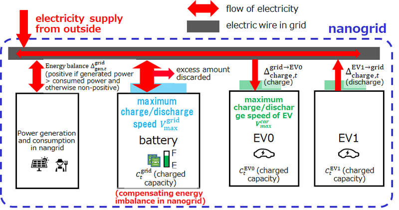
In this problem, you operate multiple electric vehicles (EVs) to protect distributed nanogrids from overloading the electrical supply to EVs and to provide additional power from EVs if there is a power shortage in the nanogrids. Since EVs consume electricity proportional to their distances traveled, they need to charge from nanogrids if necessary. Each nanogrid is equipped with a battery, a photovoltaic (PV) power system and a fuel engine. Power generation, consumption and charge/discharge to EVs occur in each nanogrid and their time-varying imbalance is compensated by charge/discharge from the battery and electrical supply from outside.

The toolkit, which can be downloaded from the bottom of this page, contains a sample of contestant code in which input/output such as reading data from the judge code has already been implemented. Also, regarding the operation of EV, "all stay" and "random walk" have been implemented as examples. When implementing a new algorithm, the sample is designed so that you can focus on describing the operation of EV by inheriting the strategy class. (See README.md for details.) You can use the sample when submitting your code.
Time Schedules and Spatial Structures
- Time Schedules: The total time length of each test case corresponds physically to one business day. The time variable t is supposed to be integer valued ranging from 0 to T_{max}. For each test case, one of the four different one day weather patterns is randomly assigned and the weather pattern affects the resulting time series of difference between generated and consumed powers (energy balance). In the beginning of each test case, each contestant gets a whole time series of predicted energy balance and, for each time t, each contestant gets the charged capacity of the battery for each nanogrid, the set of orders assigned so far, and the following values in the previous step: actual energy balance, excess amount of power discarded, and power supplied from the outside. Based on the information, each contestant is asked to decide how to operate multiple EVs in the next step for each time t.
- Spatial Structures: Let G = (V, E) be a simple and undirected graph with the vertex set V and the edge set E, which represents a road network on which EV movement and EV charge/discharge occur. Nanogrids are located on some of the vertices. An edge represents the road connecting its two endpoints and has a positive integer weight corresponding to the road distance. The graph is generated by the algorithm below.
Algorithm to generate the graph G
For all test cases, the graph G = (V, E) is generated by the following algorithm.- Input:|V|, |E|, \mathrm{MaxDegree}=5
- Algorithm to generate the vertices:
- Find the maximum non-negative integer R such that |V| = R^{2} + r holds for a non-negative integer r.
- For each lattice point satisfying 0 \leq x, y < R in the xy plane, plot a point (x, y).
- Shift each point such as (x, y) \leftarrow (x + dx, y + dy) where dx and dy are random numbers sampled uniformly from the interval [0, 1].
- Remaining r points are plotted at (x', y') where x' and y' are random numbers sampled uniformly from the interval [0, R].
- Assign a separate ID ranging from 1 to |V| to each point and identify each point to the vertex having the assigned ID.
- Algorithm to generate the |V|-1 edges and their weights to guarantee the connectivity of the resulting graph:
- Generate the complete graph G_{\text{comp}} with the vertex set V. For each pair of vertices u, v \in V, assign the Euclidean distance between the points corresponding to u and v to the edge weight W_{u,v}.
- Generate the minimum spanning tree for G_{\text{comp}} and add |V|-1 edges in the minimum spanning tree to the graph G. For each edge \left\{ u, v \right\}, assign \lceil 2 \times W_{u, v} \rceil to the edge weight d_{u,v}.
- Algorithm to generate the remaining |E|-(|V|-1) edges and their weights:
- Remaining |E|-(|V|-1) edges are generated by the following algorithm.
- Update \mathrm{cost}(u,v) based on the algorithm below.
- Find the pair of vertices u and v minimizing \mathrm{cost(u,v)} among all the pairs of vertices not connected by the edges added to the graph G so far and add the edge \left\{ u, v \right\} connecting the pair to the graph G.
- Assign \lceil 2 \times W_{u, v} \rceil to the edge weight d_{u,v}.
-
Here \mathrm{cost}(u,v) is basically determined by the Euclidean distance between the points corresponding to u and v but is biased so that a pair of vertices u and v one of whose degree is small and a pair of vertices lining up vertically and horizontally rather than diagonally are likely to be selected. Due to the bias, the resulting graph is expected to be close to a planer graph. In what follows, we show the algorithm to compute \mathrm{cost}(u,v).
- Compute the degree \mathrm{degree}(u) of the vertex u\in V. The degree \mathrm{degree}(u) of the vertex u\in V is defined by the number of edges incident to the vertex.
- Assign a color to each vertex u\in V as follows: Colors of the first added R^{2} vertices are determined based on their original lattice points (x,y) based on the rule below. Colors of the remaining r vertices are randomly assigned to be 0 or 1.
- If x+y is even : \mathrm{color}(u) = 0
- If x+y is odd : \mathrm{color}(u) = 1
- Bias factor f(u,v) is determined by the following rule:
- If \mathrm{color}(u) = \mathrm{color}(v) : \mathrm{f}(u,v) = 5
- If \mathrm{color}(u) \neq \mathrm{color}(v) : \mathrm{f}(u,v) = 1
- Bias factor g(u) is determined by the following rule:
- If \mathrm{degree}(u) \lt \mathrm{MaxDegree} : g(u)=1
- If \mathrm{degree}(u) \geq \mathrm{MaxDegree} : g(u)=\infty
- Compute \mathrm{cost}(u,v) as follows:
- \mathrm{cost}(u,v) = W_{u,v}\times \mathrm{degree}(u) \times \mathrm{degree}(v) \times f(u,v) \times g(u) \times g(v).
- Remaining |E|-(|V|-1) edges are generated by the following algorithm.
- Algorithm to select vertices where nanogrids are located :
- Uniformly and randomly select N_{\mathrm{grid}} distinct vertices from V and locate a nanogrid on each selected vertex. The set of the vertices on which nanogrids are located is denoted as V_{\mathrm{grid}}.
Constitution of a Nanogrid
Each nanogrid consists of a battery, a photovoltaic (PV) power system, a fuel engine, charging/discharging stations for EVs and power consumers and has the following attributes.
-
Vertex ID: ID of the vertex u on which the nanogrid is located where u \in V_{\mathrm{grid}} (V_{\mathrm{grid}}: the set of vertices on which nanogrids are located (See "Algorithm to generate the graph G".) )
-
Charged Capacity: The charged capacity of the battery in the nanogrid. Its initial value is C_{\mathrm{init}}^{\mathrm{grid}} and its maximum value is C_{\mathrm{max}}^{\mathrm{grid}}, which are the same for all the nanogrids. For each time t, the charged capacity changes by the difference between generated and consumed powers (energy balance) and it also changes by the difference between discharged and charged electricity to EVs (For the detail, see Charge/Discharge to the Battery of a Nanogrid .). If the resulting charged capacity exceeds C_{\mathrm{max}}^{\mathrm{grid}} at the time t, the charged capacity is set to C_{\mathrm{max}}^{\mathrm{grid}} at the time t+1 and the excess amount is discarded. Instead, if the resulting capacity is negative at the time t, the shortage is supplied from outside and the charged capacity is set to 0 at the time t+1. If the latter is the case, the score is deducted in proportion to the amount of shortage (For the detail, see Scoring.)
-
Energy Balance: Difference between generated and consumed powers except for those for charging/discharging EVs for each time t. Its predicted value for each time t is provided to contestants in the beginning of each test case. Its actual value is sums of the predicted value and random value caused by stochastic fluctuation of the environment and sudden weather changes like downpour and sudden clear sky (For the detail, see Energy Balance below.)
-
Maximum charging/discharging speed: The maximum speed of charging/discharging to the battery V_{\max}^{\mathrm{grid}}, which is the same for all the nanogrids.
Energy Balance
Difference between generated and consumed powers except for those for charging/discharging EVs for each time t.
-
Pattern of the time series of the energy balance: For each test case, one of the four different one day weather patterns, i.e., sunny with/without downpour and rainy with/without sudden clear sky is randomly assigned and is informed to each contestant in the beginning of the test case. For each nanogrid, one of the N_{\mathrm{pattern}} different expected demand patterns is randomly assigned and is informed to each contestant in the beginning of each test case. A whole time series of predicted energy balance is provided to each contestant in the beginning of each test case. The amount of generated powers from the PV power system depends on the weather pattern and thus the sums of the predicted values of energy balance in one business day is largest for the weather pattern, sunny without downpour, and is smallest for the weather pattern, rainy without sudden clear sky.
-
The time series of the energy balance: The time series of the energy balance is sums of predicted one and stochastic fluctuation \delta and the variation due to downpour and sudden clear sky.
- The total time interval 0 \leq t < T_{\max} is divided into N_{\mathrm{div}} subintervals of equal length and predicted value of the energy balance is constant for each subdivided interval.
- For each time t, \delta is sampled from the normal distribution with the mean 0 and the variance \sigma^{2}_{\mathrm{ele}}. The variance is informed to each contestant in the beginning of each test case but the value \delta is not informed to each contestant in advance.
- Downpour: If the weather pattern is 1 (sunny with downpour), downpour occurs with a probability p_{\mathrm{event}} for each of N_{\mathrm{div}} subintervals. The probability is constant and independent for each subinterval. If the downpour occurs, the energy balance is subtracted by \Delta_{\mathrm{event}} for 15 percent of the nanogrids randomly and independently chosen for each subinterval because generated power from a photovoltaic (PV) power system decreases.
- Sudden clear sky: If the weather pattern is 3 (rainy with sudden clear sky), sudden clear sky occurs with the probability p_{\mathrm{event}} for each of the N_{\mathrm{div}} subintervals. If the sudden clear sky occurs, the energy balance is added by \Delta_{\mathrm{event}} for 15 percent of the nanogrids randomly and independently chosen for each subinterval because generated power from a photovoltaic (PV) power system increases.
In case of the weather patterns 1 and 3, the timing for downpour or sudden clear sky is not informed to each contestant in advance.

EV Operation
Each contestant is asked to operate multiple electric vehicles (EVs) to protect distributed nanogrids from overloading the electrical supply to EVs and to provide additional power from EVs if there is a power shortage in the nanogrids.
-
Number of EVs: The number of EVs N^{\mathrm{EV}} is uniformly randomly selected from the interval [N_{\min}^{\mathrm{EV}}, N_{\max}^{\mathrm{EV}}] and is informed to each contestant in the beginning of each test case.
-
Initial Position of EVs: In the beginning of each test case, N^{\mathrm{EV}} vertices are selected randomly and one EV is placed on each selected vertex.
-
Attributes for EV: Each EV has the following attributes:
- ID (0, 1,... , N^{\mathrm{EV}}-1)
- Charged capacity: C^{\mathrm{EV}}_{t} non-negative integer valued, initialized to C^{\mathrm{EV}}_{t=0}, and has the upper limit C^{\mathrm{EV}}_{\max} common for all the EVs
- Present location: either on a vertex or on an edge
- Maximum charging/discharging speed: V_{\max}^{\mathrm{EV}}, which is common for all the EVs.
-
Operation for EVs: For each time t, each contestant chooses one of the operations below for each EV:
stay: Let the EV stay in the same place. In this case, the EV does not consume electricity, i.e., C^{\mathrm{EV}}_{t+1}-C^{\mathrm{EV}}_{t}=0.-
move w: Let the EV move forward to the vertex w \in V by the distance 1. The charged capacity of the EV in the next step decreases by \Delta^{\mathrm{EV}}_{\mathrm{move}} unless the resulting charged capacity is negative. If that is the case, the operation is rejected, the EV stays at the same position and its charged capacity does not change if the following conditions are satisfied.- Suppose the operation
move wis selected. Then, each contestant getsWA(Wrong Answer) if one of the conditions below are violated.- w \in V
- Supposing the present position of the EV is on u \in V, \left\{ u, w \right\} \in E holds.
- Supposing the present position of the EV is on \left\{ u, v \right\}, w = u or w = v holds.
- Suppose the operation
-
charge_from_grid\Delta^{\mathrm{grid} \rightarrow \mathrm{EV}}_{\mathrm{charge}}: Charge the EV by \Delta^{\mathrm{grid} \rightarrow \mathrm{EV}}_{\mathrm{charge}}. The charged capacity of the EV in the next step C^{\mathrm{EV}}_{t+1} becomes C^{\mathrm{EV}}_{t+1} \leftarrow C^{\mathrm{EV}}_{t} + \Delta^{\mathrm{grid} \rightarrow \mathrm{EV}}_{\mathrm{charge},t}. It is possible to charge multiple EVs from a single nanogrid.- Suppose the operation
charge_from_gridis selected with \Delta^{\mathrm{grid} \rightarrow \mathrm{EV}}_{\mathrm{charge}}. Then, each contestant getsWA(Wrong Answer) if one of the conditions below is violated.- EV is on a vertex where a nanogrid is located u \in V_{\mathrm{grid}}.
- \Delta^{\mathrm{grid} \rightarrow \mathrm{EV}}_{\mathrm{charge}} is a natural number.
- Charged amount for each EV does not exceed the maximum charge/discharge speed: \Delta^{\mathrm{grid} \rightarrow \mathrm{EV}}_{\mathrm{charge}} \leq V_{\max}^{\mathrm{EV}}
- The resulting charged capacity for each EV does not exceed the upper limit C^{\mathrm{EV}}_{\max}: C^{\mathrm{EV}}_{t} + \Delta^{\mathrm{grid} \rightarrow \mathrm{EV}}_{\mathrm{charge}} \leq C^{\mathrm{EV}}_{\max}
- Suppose the operation
-
charge_to_grid\Delta^{\mathrm{EV} \rightarrow \mathrm{grid}}_{\mathrm{charge}}: Charge a nanogrid from the EV by \Delta^{\mathrm{EV} \rightarrow \mathrm{grid}}_{\mathrm{charge}}. The charged capacity of the EV in the next step C^{\mathrm{EV}}_{t+1} becomes C^{\mathrm{EV}}_{t+1} \leftarrow C^{\mathrm{EV}}_{t} - \Delta^{\mathrm{EV} \rightarrow \mathrm{grid}}_{\mathrm{charge},t}. It is possible to charge a nanogrid from multiple EVs. It is also possible to charge EVs from a nanogrid and charge the nanogrid from other EVs simultaneously.- Suppose the operation
charge_to_gridis selected with \Delta^{\mathrm{EV} \rightarrow \mathrm{grid}}_{\mathrm{charge}}. Then, each contestant getsWA(Wrong Answer) if one of the conditions below is violated.- EV is on a vertex where a nanogrid is located u \in V_{\mathrm{grid}}.
- \Delta^{\mathrm{EV} \rightarrow \mathrm{grid}}_{\mathrm{charge}} is a natural number.
- Charged amount for each EV does not exceed the maximum charge/discharge speed: \Delta^{\mathrm{EV} \rightarrow \mathrm{grid}}_{\mathrm{charge}} \leq V_{\max}^{\mathrm{EV}}
- The resulting charged capacity for each EV is not negative: C^{\mathrm{EV}}_{t} - \Delta^{\mathrm{EV} \rightarrow \mathrm{grid}}_{\mathrm{charge}} \geq 0
- Suppose the operation
Charge/Discharge to the Battery of a Nanogrid
For each nanogrid, the charged capacity of the battery varies in time depending on the difference between generated and consumed powers and the amount of charge/discharge to EVs. For each time t, sums of the difference between generated and consumed powers and gross difference between charged/discharged amounts to EVs from the nanogrid correspond to power excess or shortage in the nanogrid. If the power excess occurs, the battery is charged by the amount provided that the power excess does not exceed the maximum charge speed of the battery and the resulting charged capacity of the battery does not exceed its upper limit. If the power excess exceeds the maximum charge speed of the battery, the excess amount is discarded and the battery is charged by the maximum charge speed. If the resulting charged capacity of the battery exceeds its upper limit, the charged capacity is set to the upper limit at the next step and the excess amount is discarded. If the power shortage occurs instead, the power shortage is compensated by discharging the battery provided that the power shortage does not fall below the maximum discharge speed of the battery and the resulting charged capacity of the battery is not negative. If the power shortage falls below the maximum discharge speed of the battery, the power shortage is covered by discharging the battery by the maximum discharge speed and by power supplied from the outside. If the resulting charged capacity of the battery is negative, the charged capacity of the battery is set to zero in the next step and shortage is supplied from the outside. In all the cases, each EV is charged or discharged by the amount prescribed by each contestant.
Algorithm to determine an amount of charge/discharge to the battery in the next step consists of the following 4 steps.
-
Step 1: Compute the power excess or shortage in each nanogrid at time t \Delta^{\mathrm{grid}}_{\mathrm{total}}.
\Delta^{\mathrm{grid}}_{\mathrm{total}} = \Delta^{\mathrm{grid}}_{\mathrm{gen},t} - \sum_{i \in \mathrm{all EV}} \Delta^{\mathrm{grid} \rightarrow \mathrm{EV}i}_{\mathrm{charge},t} + \sum_{i \in \mathrm{all EV}} \Delta^{\mathrm{EV}i \rightarrow \mathrm{grid}}_{\mathrm{charge},t}
Here, each variable is defined as follows.- \Delta^{\mathrm{grid}}_{\mathrm{gen},t}: the difference between generated and consumed powers at the nanogrid at the time t, which is sums of predicted difference between generated and consumed powers \Delta^{\mathrm{grid,predict}}_{\mathrm{gen},t}, a stochastic fluctuation \delta_{t}, and the variation due to downpour and sudden clear sky. Note that the time series of predicted difference between generated and consumed powers is informed to each contestant in the beginning of each test case but the stochastic fluctuation is not informed until the time t (informed at the next time step t+1).
- \Delta^{\mathrm{grid} \rightarrow \mathrm{EV}i}_{\mathrm{charge},t}: Charged amount to the i-th EV from the nanogrid prescribed by the contestant at the time t
- \Delta^{\mathrm{EV}i \rightarrow \mathrm{grid}}_{\mathrm{charge},t}: Charged amount to the nanogrid from the i-th EV prescribed by the contestant at the time t
-
Step 2: In case of \Delta^{\mathrm{grid}}_{\mathrm{total}} \geq \min \left\{ V_{\max}^{\mathrm{grid}}, C^{\mathrm{grid}}_{\max}-C^{\mathrm{grid}}_{t} \right\},
The charged capacity of the nanogrid at the time t+1 is determined by the following equation:
C^{\mathrm{grid}}_{t+1} \leftarrow C^{\mathrm{grid}}_{t}+\min \left\{ V_{\max}^{\mathrm{grid}}, C^{\mathrm{grid}}_{\max}-C^{\mathrm{grid}}_{t} \right\}
Physically, this means if the power excess exceeds the maximum charge/discharge speed or the remaining capacity of the battery, the excess amount is discarded. -
Step 3: In case of \Delta^{\mathrm{grid}}_{\mathrm{total}} < - \min \left\{ V_{\max}^{\mathrm{grid}}, C^{\mathrm{grid}}_{t} \right\},
The charged capacity of the nanogrid at the time t+1 is determined by the following equation:
C^{\mathrm{grid}}_{t+1} \leftarrow C^{\mathrm{grid}}_{t} - \min \left\{ V_{\max}^{\mathrm{grid}}, C^{\mathrm{grid}}_{t} \right\}
If the power shortage cannot be compensated by discharging the battery, the remaining shortage:
L_t = - \Delta^{\mathrm{grid}}_{\mathrm{total}} - \min \left\{ V_{\max}^{\mathrm{grid}}, C^{\mathrm{grid}}_{t} \right\}(>0)
is supplied from the outside. In this case, the score is deducted in proportion to the supplied electricity with a factor \gamma. (For the detail, see Scoring.)。 -
Step 4: The other cases than the cases in step 2 and 3,
The charged capacity of the nanogrid at the time t+1 is determined by the following equation:
C^{\mathrm{grid}}_{t+1} \leftarrow C^{\mathrm{grid}}_{t} + \Delta^{\mathrm{grid}}_{\mathrm{total}}
Scoring
-
During the contest the total score of a submission is determined by summing the score of the submission with respect to 16 test cases. Among these test cases, the numbers of sunny without downpour, sunny with downpour, rainy without sudden clear sky, and rainy with sudden clear sky are fixed at 6, 2, 6, and 2, respectively.
-
The score is computed by the following equation.
\mathrm{Score}=\sum_{i=1}^{N_{\mathrm{EV}}} C_{t=T_{\max}}^{\mathrm{EV}i} + \sum_{i=1}^{N_{\mathrm{grid}}} C_{t=T_{\max}}^{\mathrm{grid}i} - \gamma \sum_{t=0}^{T_{\max}-1} \sum_{i=1}^{N_{\mathrm{grid}}} L_{i,t} + 3000000
Here, the first and the second terms in the equation are the charged capacity of all the EVs and nanogrid at the time t=T_{\max}, respectively. L_{i,t} is power supplied from the outside at the i-th grid at the time t and \gamma is a proportional constant of the penalty and L_{i,t}. The value of L_{i,t} is set to L_{i,t} = - \Delta^{\mathrm{grid}}_{\mathrm{total}} - \min \left\{ V_{\max}^{\mathrm{grid}}, C^{\mathrm{grid}}_{t} \right\}(L_{i,t}>0) if the step 3 is executed in Charge/Discharge to the Battery of a Nanogrid and is set to L_{i,t}=0 in the other cases. -
After the contest a system test will be performed. To this end, the contestant's last submission will be scored by summing the final score of the submission on 200 previously unseen test cases.
Please see the table below for a breakdown of the 200 test cases.
| Predicted energy balance (disclosed) | Predicted energy balance (undisclosed) | Total | |
|---|---|---|---|
| Sunny without downpour | 60 | 15 | 75 |
| Sunny with downpour | 20 | 5 | 25 |
| Rainy without sudden clear sky | 60 | 15 | 75 |
| Rainy with sudden clear sky | 20 | 5 | 25 |
| Total | 160 | 40 | 200 |
Of the 200 test cases, 160 use 6(=N_\mathrm{pattern} \times 2(sunny, rainy)) types of predicted energy balance already disclosed in the toolkit. The remaining 40 test cases use 6(=N_\mathrm{pattern} \times 2(sunny, rainy)) types of predicted energy balance that are not disclosed to the contestants. \Delta_{\mathrm{event}}, p_{\mathrm{event}}, and percentage of nanogrids hit by downpour or sudden clear sky are all the same among 50(=25[sunny with downpour]+25[rainy with sudden clear sky]) test cases.
We are very sorry that the system test specifications have changed unlike the answer to the question received from Mr. yuusanlondon on December 18.
As a result of consideration, the organizers of the contest have determined to decide the final standings based on this specification. We appreciate your understanding.
(12/29 postscript) Generation method or generator for undisclosed predicted energy balance will not be released. Patterns of undisclosed predicted energy balance are generated so that the full score for Electricity Management using undisclosed predicted energy balance is comparable to that using disclosed predicted energy balance. (Note that the full score means the upper limit of the score by applying an ideal control method.)
Problem A
Problem A is an interactive problem. To obtain a high score, each contestant is asked to operate (charge/discharge) multiple EVs so that there is no excess or deficiency in the charged capacity of the battery in each nanogrid depending on the energy balance that fluctuates stochastically. Each contestant and a host machine (judge) interact with the following protocol.
| Iterative process | Contestant | Judge |
|---|---|---|
| Output G | ||
| Output the weather \mathrm{DayType} | ||
| Output the information related to energy balance | ||
| Output the information about the nanogrid | ||
| Output the information about EV | ||
| Output the information about the score | ||
| Output T_\mathrm{max} | ||
| for t=0,...,T_\mathrm{max}-1 do | - | - |
| Output \mathrm{info}_t (the status of EVs and nanogrids at the time t) | ||
| Output operations for each EV | ||
| end for | ||
| Output \mathrm{info}_t (the status of EVs and nanogrids at the time t=T_\mathrm{max}) | ||
| Output score \mathrm{Score} |
The graph G, the weather \mathrm{DayType}, the information related to energy balance, the nanogrid, EVs, the score, and T_\mathrm{max} are outputted only once in the beginning of each test case. For each test case, contestants are supposed to interact with judges T_\mathrm{max} times. Note that \mathrm{info}_t and the score at the time t=T_\mathrm{max} must be read by the contestant code (otherwise it may be TLE).
Input and Output Format 1
In the beginning of each test case, the graph G, the weather \mathrm{DayType}, the information related to energy balance, the nanogrid, EVs, the score, and T_\mathrm{max} are provided through the standard input.
|V| |E|
u_1 v_1 d_1
:
u_{|E|} v_{|E|} d_{|E|}
\mathrm{DayType}
N_\mathrm{div} N_\mathrm{pattern} \sigma^{2}_{\mathrm{ele}} p_{\mathrm{event}} \Delta_{\mathrm{event}}
\mathrm{pw}_{1,1}^{\mathrm{predict}} \mathrm{pw}_{1,2}^{\mathrm{predict}} ... \mathrm{pw}_{1,N_\mathrm{div}}^{\mathrm{predict}}
:
\mathrm{pw}_{N_\mathrm{pattern},1}^{\mathrm{predict}} \mathrm{pw}_{N_\mathrm{pattern},2}^{\mathrm{predict}} ... \mathrm{pw}_{N_\mathrm{pattern},N_\mathrm{div}}^{\mathrm{predict}}
N_\mathrm{grid} C_{\mathrm{init}}^{\mathrm{grid}} C_{\mathrm{max}}^{\mathrm{grid}} V_{\max}^{\mathrm{grid}}
x_1 \mathrm{pattern}_1
:
x_{N_\mathrm{grid}} \mathrm{pattern}_{N_\mathrm{grid}}
N_\mathrm{EV} C_{\mathrm{init}}^{\mathrm{EV}} C_{\mathrm{max}}^{\mathrm{EV}} V_{\max}^{\mathrm{EV}} \Delta_{\mathrm{move}}^{\mathrm{EV}}
\mathrm{pos}_1
:
\mathrm{pos}_{N_\mathrm{EV}}
\gamma
T_\mathrm{max}
- In the 1st line, the number of vertices |V| and the number of edges |E| of the graph G are provided.
- In the following |E| lines, the edges of the graph along with their weights are provided. The i-th line of the lines indicate that there exists an edge connecting u_{i} and v_{i} with the edge weight d_i.
- In the following 1 line, the weather pattern \mathrm{DayType} is provided, which is either \mathrm{DayType} 0 (sunny without downpour), 1 (sunny with downpour), 2 (rainy without sudden clear sky), or 3 (rainy with sudden clear sky).
- In the following 1 line, the number of subintervals of equal length on which the predicted energy balance is constant N_\mathrm{div}, the number of possible patterns of the time series of predicted energy balance N_\mathrm{pattern}, the variance of the stochastic fluctuation of the difference \sigma^{2}_{\mathrm{ele}}, the probability of occurrences of downpour or sudden clear p_{\mathrm{event}} (p_{\mathrm{event}}=0.0 in the case of \mathrm{DayType}=0 or 2), and the variation of energy balance in case of downpour or sudden clear sky \Delta_{\mathrm{event}}.
- In the following N_\mathrm{pattern} lines, the time series of predicted energy balance is provided. The j-th element in the i-th line of the lines (\mathrm{pw}_{i,j}^{\mathrm{predict}}) indicates the predicted energy balance of the j-th subinterval in case of the i-th pattern.
- In the following 1 line, the number of nanogrids N_\mathrm{grid} and the initial value of the charged capacity of the battery for each nanogrid C_{\mathrm{init}}^{\mathrm{grid}} (t=0), the upper limit of the charged capacity of the battery C_{\mathrm{max}}^{\mathrm{grid}}, and the maximum charge/discharge speed of the battery V_{\max}^{\mathrm{grid}} is provided.
- In the following N_\mathrm{grid} lines, the information about each nanogrid is provided. In the N_\mathrm{grid} lines, the i-th line indicates that a nanogrid is located on the vertex x_i whose pattern of the time series of predicted energy balance is \mathrm{pattern}_i.
- In the following 1 line, the number of EVs N_\mathrm{EV}, their initial charged capacity C_{\mathrm{init}}^{\mathrm{EV}}, their maximum charged capacity C_{\mathrm{max}}^{\mathrm{EV}}, and their maximum charge/discharge speed V_{\max}^{\mathrm{EV}}, and the amount of electricity necessary for each EV to travel in a unit distance \Delta_{\mathrm{move}}^{\mathrm{EV}}.
- In the following N_\mathrm{EV} lines, the position of each EV is provided. In the N_\mathrm{EV} line, the i-th line indicates that the i-th EV is located on the vertex \mathrm{pos}_i.
- In the following 1 line, the proportional constant \gamma for the penalty of getting power supply from outside is provided.
- In the last line, the total time step for each trial of each test case T_{\max} is provided.
Input and Output Format 2
For each time t, contestants get the status of EVs and nanogrids \mathrm{info}_t from the standard input.
x_1 y_1 \mathrm{pw}_{1}^{\mathrm{actual},t-1} \mathrm{pw}_{1}^{\mathrm{excess},t-1} \mathrm{pw}_{1}^{\mathrm{buy},t-1}
:
x_{N_\mathrm{grid}} y_{N_\mathrm{grid}} \mathrm{pw}_{N_\mathrm{grid}}^{\mathrm{actual},t-1} \mathrm{pw}_{N_\mathrm{grid}}^{\mathrm{excess},t-1} \mathrm{pw}_{N_\mathrm{grid}}^{\mathrm{buy},t-1}
\mathrm{carinfo}_1
:
\mathrm{carinfo}_{N_\mathrm{EV}}
- In the N_\mathrm{grid} lines, the i-th line indicates the charged capacity of the battery of the nanogrid on the vertex x_i is y_i, and \mathrm{pw}_{i}^{\mathrm{actual},t-1}, \mathrm{pw}_{i}^{\mathrm{excess},t-1}, and \mathrm{pw}_{i}^{\mathrm{buy},t-1} indicate actual energy balance, excess amount of power discarded, and power supplied from the outside at the previous time step t-1, respectively. At t=0, \mathrm{pw}_{i}^{\mathrm{actual},t-1}, \mathrm{pw}_{i}^{\mathrm{excess},t-1}, and \mathrm{pw}_{i}^{\mathrm{buy},t-1} are all displayed as 0.
Note that \mathrm{pw}_{i}^{\mathrm{actual},t-1}, \mathrm{pw}_{i}^{\mathrm{excess},t-1}, and \mathrm{pw}_{i}^{\mathrm{buy},t-1} correspond to \Delta^{\mathrm{grid}}_{\mathrm{gen},t-1}, \Delta^{\mathrm{grid}}_{\mathrm{total},t-1} - \min \left\{ V_{\max}^{\mathrm{grid}}, C^{\mathrm{grid}}_{\max}-C^{\mathrm{grid}}_{t-1} \right\}, and - \Delta^{\mathrm{grid}}_{\mathrm{total},t-1} - \min \left\{ V_{\max}^{\mathrm{grid}}, C^{\mathrm{grid}}_{t-1} \right\}, respectively (see Charge/Discharge to the Battery of a Nanogrid ).
If "step 2" and "step 3" are not executed at the previous time t−1, \mathrm{pw}_{i}^{\mathrm{excess},t-1} and \mathrm{pw}_{i}^{\mathrm{buy},t-1} are 0, respectively. - In the following N_\mathrm{EV} groups of 3 lines, the i-th group \mathrm{carinfo}_i indicated the status of the i-th EV. For the detail, see the information below.
Here, \mathrm{carinfo}_i is provided in the following format.
\mathrm{charge}_i
u_i v_i \mathrm{dist\_from}\_u_i \mathrm{dist\_to}\_v_i
N_{\mathrm{adj},i} a_{i,1} a_{i,2} \ldots a_{i,N_\mathrm{adj}}
- The first line indicates that the charged capacity of the i-th EV is \mathrm{charge}_i.
- The second line indicates the present position of i-th. If u_i \ne v_i holds, the i-th EV is on the edge connecting u_i and v_i, and the distance to the vertex u_i is \mathrm{dist\_from}\_u_i and that to v_i is \mathrm{dist\_to}\_v_i. If u_i = v_i holds, the i-th EV is on the vertex u_i (in this case, both \mathrm{dist\_from}\_u_i and \mathrm{dist\_to}\_v_i are displayed as 0).
- The third line indicates that there are N_{\mathrm{adj},i} possible vertices to which the i EV moves by the operation
moveand a_{i,1}, a_{i,2}、\ldots and a_{i,N_\mathrm{adj}} are the possible vertices.
In responding to the input, contestants are asked to output the operation of each EV \mathrm{command}_i (1 \leq i \leq N_\mathrm{EV}) for each time t (0 \leq t \lt T_{\max}). Each operation should be separated by the new line and the output should end with the new line.
\mathrm{command}_{1}
\mathrm{command}_{2}
:
\mathrm{command}_{N_\mathrm{EV}}
Here, \mathrm{command} should be in the following format. There are four possible operations stay, move w, charge_from_grid, and charge_to_grid for each EV. Contestants should choose one of them for each EV and output it in one line as follows:
staymove wcharge_from_grid\Delta^{\mathrm{grid} \rightarrow \mathrm{EV}}_{\mathrm{charge}}charge_to_grid\Delta^{\mathrm{EV} \rightarrow \mathrm{grid}}_{\mathrm{charge}}
There are constraints for each operation (See EV Operation for EVs for the detail). The behavior of the judge when one of these constraints is violated is undefined.
Input and Output Format 3
After the operation of each EV at t=T_\mathrm{max}-1 is output, \mathrm{info}_t at t=T_\mathrm{max} is provided through the standard input from the judge (the format of \mathrm{info}_t is the same as the format written in Input/Output format 2). On the next line, then, the judge gives the score to the standard input in the following format.
\mathrm{Score}
Constraints for Input and Output
- Of the following numbers, those described as "[float]" are given as floats, and the others are given as integers.
Input and output format 1 provided in the beginning of each test case
- |V| = 225
- 1.5 |V| \leq |E| \leq 2 |V|
- 1 \leq u_{i}, v_{i} \leq |V|, u_i \ne v_i (1 \leq i \leq |E|)
- 1 \leq d_i \leq \lceil 2\sqrt{2|V|} \rceil (1 \leq i \leq |E|)
- The graph G is guaranteed to be simple and connected.
- \mathrm{DayType} \in \left\{ 0, 1, 2, 3 \right\}
- N_\mathrm{div} = 20
- N_\mathrm{pattern} = 3
- \sigma^{2}_{\mathrm{ele}} = 100
- p_{\mathrm{event}} \in \left\{ 0.0, 0.1 \right\} "[float]"
- \Delta_{\mathrm{event}} = 1000
- -1000 \lt \mathrm{pw}_{i,j}^{\mathrm{predict}} \lt 1000 (1 \leq i \leq N_\mathrm{pattern}, 1 \leq j \leq N_\mathrm{div})
- N_\mathrm{grid} = 20
- C_{\mathrm{init}}^{\mathrm{grid}} = 25000
- C_{\mathrm{max}}^{\mathrm{grid}} = 50000
- V_{\max}^{\mathrm{grid}} = 800
- 1 \leq x_i \leq |V| (if i \neq j, x_i \neq x_j. 1 \leq i \leq N_\mathrm{grid})
- 1 \leq \mathrm{pattern}_i \leq N_\mathrm{pattern} (1 \leq i \leq N_\mathrm{grid})
- N_{\min}^{\mathrm{EV}} = 15
- N_{\max}^{\mathrm{EV}} = 25
- N_{\min}^{\mathrm{EV}} \leq N_\mathrm{EV} \leq N_{\max}^{\mathrm{EV}}
- C_{\mathrm{init}}^{\mathrm{EV}} = 12500
- C_{\mathrm{max}}^{\mathrm{EV}} = 25000
- V_{\max}^{\mathrm{EV}} = 400
- \Delta_{\mathrm{move}}^{\mathrm{EV}} = 50
- 1 \leq \mathrm{pos}_i \leq |V| (1 \leq i \leq N_\mathrm{EV})
- \gamma = 2.0 "[float]"
- T_\mathrm{max} = 1000
Input and output format 2 provided for each time step
- 1 \leq x_i \leq |V| (if i \neq j, x_i \neq x_j. 1 \leq i \leq N_\mathrm{grid})
- 0 \leq y_i \leq C_{\mathrm{max}}^{\mathrm{grid}} (1 \leq i \leq N_\mathrm{grid})
- -10000 \lt \mathrm{pw}_{i}^{\mathrm{actual},j} \lt 10000 (1 \leq i \leq N_\mathrm{grid}, -1 \leq j \leq T_\mathrm{max}-2)
- 0 \leq \mathrm{pw}_{i}^{\mathrm{excess},j} \lt 10000, (1 \leq i \leq N_\mathrm{grid}, -1 \leq j \leq T_\mathrm{max}-2)
- 0 \leq \mathrm{pw}_{i}^{\mathrm{buy},j} \lt 10000, (1 \leq i \leq N_\mathrm{grid}, -1 \leq j \leq T_\mathrm{max}-2)
- 0 \leq \mathrm{charge}_i \leq C_{\mathrm{max}}^{\mathrm{EV}} (1 \leq i \leq N_\mathrm{EV})
- 1 \leq u_i, v_i \leq |V| (1 \leq i \leq N_\mathrm{EV})
- 0 \leq \mathrm{dist\_from}\_u_i \leq \lceil 2\sqrt{2|V|} \rceil (1 \leq i \leq N_\mathrm{EV})
- 0 \leq \mathrm{dist\_to}\_v_i \leq \lceil 2\sqrt{2|V|} \rceil (1 \leq i \leq N_\mathrm{EV})
- 1 \leq N_{\mathrm{adj},i} \leq 5(\mathrm{MaxDegree}) (1 \leq i \leq N_\mathrm{EV})
- 1 \leq a_{i,j} \leq |V| (1 \leq i \leq N_\mathrm{EV}, 1 \leq j \leq N_{\mathrm{adj},i})
Input and output format 3 provided at the end of each test case
- \mathrm{Score} "[float]"
Example of Inputs and Outputs
Note: This example is to explain how a judge and a contestant interact with each other through inputs and outputs. To simplify the explanation, some of the parameter values like the number of vertices are set to small and they may be outside of the ranges in Constraints of Input and Output. For example, the number of vertices is set to 4 in this example but is set to 225 in each test case.
| Time Step | Judge | Contestant | Explanation |
|---|---|---|---|
4 4 1 2 1 2 3 2 3 4 3 4 1 1 0 2 2 1 0 10 5 -2 -4 4 2 10 20 4 1 1 4 2 2 5 10 2 1 2 4 0.5 4 |
Initial parameter values are provided by Judge in the beginning of each test case Line 1: Graph G consists of |V| = 4 vertices and |E| = 4 edges. The following 4 lines (Line 2 - Line 5) indicate the edges of the graph. Line 2: Edge 1 connects the vertex 1 and 2 and its distance is 1. Line 3: Edge 2 connects the vertex 2 and 3 and its distance is 2. Line 4: Edge 3 connects the vertex 3 and 4 and its distance is 3. Line 5: Edge 4 connects the vertex 4 and 1 and its distance is 1. Line 6: The weather pattern in this test case is 0 "Sunny without downpour". Line 7: N_{\mathrm{div}} is 2, N_\mathrm{pattern} is 2, \sigma^{2}_{\mathrm{ele}} is 1, p_{\mathrm{event}} is 0, \Delta_{\mathrm{event}} is 10. The following 2 lines (Line 9 - Line 10) indicate the predicted energy balance. Line 8: The predicted energy balance of nanogrids having the demand pattern 1 is 5 for the 1st time interval and -2 for the 2nd time interval. Line 9: The predicted energy balance of nanogrids having the demand pattern 1 is -4 for the 1st time interval and 4 for the 2nd time interval. Line 10: N_\mathrm{grid} = 2, C_{\mathrm{init}}^{\mathrm{grid}} = 10, C_{\mathrm{max}}^{\mathrm{grid}} = 20 and V_{\max}^{\mathrm{grid}} = 4. Line 11: Nanogrid 1 is on the vertex 1 and it has the demand pattern 1. Line 12: Nanogrid 2 is on the vertex 4 and it has the demand pattern 2. Line 13: N_\mathrm{EV} = 2, C_{\mathrm{init}}^{\mathrm{EV}} = 5, C_{\mathrm{max}}^{\mathrm{EV}} = 10, V_{\max}^{\mathrm{EV}} = 2, and \Delta_{\mathrm{move}}^{\mathrm{EV}} = 1. The following 2 lines (Line 14 - Line 15) indicate the positions of the EVs at time t=0. Line 14: EV 1 is on the vertex 2 at time t=0. Line 15: EV 2 is on the vertex 4 at time t=0. Line 16: \gamma = 0.5. Line 17: T_{\max} = 4. |
||
| 0 | 1 10 0 0 0 4 10 0 0 0 5 2 2 0 0 2 1 3 5 4 4 0 0 2 1 3 |
move 1 charge_from_grid 2 |
Input data at time 0 is provided by Judge. Line 1: The charged capacity of the nanogrid at the vertex 1 at time 0 is 10. All the other three values are irrelevant at time 0 and are set to 0. Line 2: The charged capacity of the nanogrid at the vertex 4 at time 0 is 10. All the other three values are irrelevant at time 0 and are set to 0. The following 3 lines (Line 3 - Line 5) indicate the status of EV 1. Line 3: The charged capacity of EV 1 is 5 at time 0. Line 4: EV 1 is on the vertex 2 at time 0. Line 5: There are N_{\mathrm{adj},1} = 2 vertices toward which EV 1 can `move` and the vertices are 1 and 3. The following 3 lines (Line 6 - Line 8) indicate the status of EV 2. Line 6: The charged capacity of EV 2 is 5 at time 0. Line 7: EV 2 is on the vertex 4 at time 0. Line 8: There are N_{\mathrm{adj},1} = 2 vertices toward which EV 2 can `move` and the vertices are 1 and 3. Output from Contestant Line 1: Operate EV 1 to move toward the vertex 1. If the charged capacity of EV 1 is less than 1, EV 1 cannot move as operated. In this case, the charged capacity of EV 1 is 5 and thus EV 1 moves toward the vertex 1 by the distance 1 by consuming electricity by 1 in the next time step. Since the road distance of the edge connecting the vertices 1 and 2 is 1, the location of EV 1 is the vertex 1 in the next time step. Line 2: EV 2 charges from the nanogrid by 2. This operation does not violate the constraints because EV 2 is on the vertex 4 where the nanogrid is located, the charged amount 2 does not exceeds the maximum charge speeds of EV. Since the resulting charged capacity of EV 2 is 7, which is less than the maximum charged capacity of EV (10), the resulting charged capacity of EV 2 is 7 in the next time step. |
| 1 | 1 14 5 1 0 4 6 -4 0 2 4 1 1 0 0 2 2 4 7 4 4 0 0 2 1 3 |
stay charge_from_grid 2 |
Input data at time 1 is provided by Judge. Line 1: The charged capacity of the nanogrid on the vertex 1 at time 1 is 14. The actual energy balance, the amount of electricity overflowed, and the amount of the electricity supplied from the outside at time 0 are 5, 1, 0 , respectively. Line 2: The charged capacity of the nanogrid on the vertex 4 at time 1 is 6. The actual energy balance, the amount of electricity overflowed, and the amount of the electricity supplied from the outside at time 0 are -4, 0, 2 , respectively. The following 3 lines (Line 3 - Line 5) indicate the status of EV 1. Line 3: The charged capacity of EV 1 is 4 at time 1. Line 4: EV 1 is on the vertex 1 at time 1. Line 5: There are N_{\mathrm{adj},1} = 2 vertices toward which EV 1 can `move` and the vertices are 2 and 4. The following 3 lines (Line 6 - Line 8) indicate the status of EV 2. Line 6: The charged capacity of EV 2 is 7 at time 1. Line 7: EV 2 is on the vertex 4 at time 1. Line 8: There are N_{\mathrm{adj},1} = 2 vertices toward which EV 2 can `move` and the vertices are 1 and 3. Output from Contestant Line 1: EV 1 stays on the same vertex. Line 2: EV 2 charges from the nanogrid by 2. This operation does not violate the constraints because EV 2 is on the vertex 4 where the nanogrid is located, the charged amount 2 does not exceeds the maximum charge speeds of EV. Since the resulting charged capacity of EV 2 is 9, which is less than the maximum charged capacity of EV (10), the resulting charged capacity of EV 2 is 9 in the next time step. |
| 2 | 1 18 5 1 0 4 2 -4 0 2 4 1 1 0 0 2 2 4 9 4 4 0 0 2 1 3 |
move 4 charge_to_grid 2 |
Input data at time 2 is provided by Judge. Line 1: The charged capacity of the nanogrid on the vertex 1 at time 2 is 18. The actual energy balance, the amount of electricity overflowed, and the amount of the electricity supplied from the outside at time 1 are 5, 1, 0 , respectively. Line 2: The charged capacity of the nanogrid on the vertex 4 at time 2 is 2. The actual energy balance, the amount of electricity overflowed, and the amount of the electricity supplied from the outside at time 1 are -4, 0, 2 , respectively. The following 3 lines (Line 3 - Line 5) indicate the status of EV 1. Line 3: The charged capacity of EV 1 is 4 at time 2. Line 4: EV 1 is on the vertex 1 at time 2. Line 5: There are N_{\mathrm{adj},1} = 2 vertices toward which EV 1 can `move` and the vertices are 2 and 4. The following 3 lines (Line 6 - Line 8) indicate the status of EV 2. Line 6: The charged capacity of EV 2 is 9 at time 2. Line 7: EV 2 is on the vertex 4 at time 2. Line 8: There are N_{\mathrm{adj},1} = 2 vertices toward which EV 2 can `move` and the vertices are 1 and 3. Output from Contestant Line 1: Operate EV 1 to move toward the vertex 4. If the charged capacity of EV 1 is less than 1, EV 1 cannot move as operated. In this case, the charged capacity of EV 1 is 4 and thus EV 1 moves toward the vertex 4 by the distance 1 by consuming electricity by 1 in the next time step. Since the road distance of the edge connecting the vertices 1 and 4 is 1, the location of EV 1 is the vertex 4 in the next time step. Line 2: EV 2 discharges to the nanogrid by 2. This operation does not violate the constraints because EV 2 is on the vertex 4 where the nanogrid is located, the discharged amount 2 does not exceeds the maximum discharge speeds of EV. Since the resulting charged capacity of EV 2 is 7, which is not negative, the resulting charged capacity of EV 2 is 7 in the next time step. |
| 3 | 1 17 -1 0 0 4 6 3 1 0 3 4 4 0 0 2 1 3 7 4 4 0 0 2 1 3 |
stay move 1 |
Input data at time 3 is provided by Judge. Line 1: The charged capacity of the nanogrid on the vertex 1 at time 3 is 17. The actual energy balance, the amount of electricity overflowed, and the amount of the electricity supplied from the outside at time 2 are -1, 0, 0 , respectively. (the predicted energy balance is -2 but the actual value is -1 because of its fluctuation.) Line 2: The charged capacity of the nanogrid on the vertex 4 at time 3 is 6. The actual energy balance, the amount of electricity overflowed, and the amount of the electricity supplied from the outside at time 2 are 3, 0, 0 , respectively. (the predicted energy balance is 4 but the actual value is 3 because of its fluctuation.) The following 3 lines (Line 3 - Line 5) indicate the status of EV 1. Line 3: The charged capacity of EV 1 is 3 at time 3. Line 4: EV 1 is on the vertex 4 at time 3. Line 5: There are N_{\mathrm{adj},1} = 2 vertices toward which EV 1 can `move` and the vertices are 1 and 3. The following 3 lines (Line 6 - Line 8) indicate the status of EV 2. Line 6: The charged capacity of EV 2 is 7 at time 3. Line 7: EV 2 is on the vertex 4 at time 3. Line 8: There are N_{\mathrm{adj},1} = 2 vertices toward which EV 2 can `move` and the vertices are 1 and 3. Output from Contestant Line 1: EV 1 stays on the same vertex. Line 2: Operate EV 2 to move toward the vertex 1. If the charged capacity of EV 2 is less than 1, EV 2 cannot move as operated. In this case, the charged capacity of EV 2 is 7 and thus EV 2 moves toward the vertex 1 by the distance 1 by consuming electricity by 1 in the next time step. Since the road distance of the edge connecting the vertices 4 and 1 is 1, the location of EV 2 is the vertex 1 in the next time step. |
| 4 | 1 15 -2 0 0 4 10 5 1 0 3 4 4 0 0 2 1 3 6 1 1 0 0 2 2 4 3000032.0 |
Input data at time 4 is provided by Judge. Line 1: The charged capacity of the nanogrid on the vertex 1 at time 4 is 15. The actual energy balance, the amount of electricity overflowed, and the amount of the electricity supplied from the outside at time 3 are -2, 0, 0 , respectively. Line 2: The charged capacity of the nanogrid on the vertex 4 at time 4 is 10. The actual energy balance, the amount of electricity overflowed, and the amount of the electricity supplied from the outside at time 3 are 5, 1, 0 , respectively. The following 3 lines (Line 3 - Line 5) indicate the status of EV 1. Line 3: The charged capacity of EV 1 is 3 at time 4. Line 4: EV 1 is on the vertex 4 at time 4. Line 5: There are N_{\mathrm{adj},1} = 2 vertices toward which EV 1 can `move` and the vertices are 1 and 3. The following 3 lines (Line 6 - Line 8) indicate the status of EV 2. Line 6: The charged capacity of EV 2 is 6 at time 4. Line 7: EV 2 is on the vertex 1 at time 4. Line 8: There are N_{\mathrm{adj},1} = 2 vertices toward which EV 2 can `move` and the vertices are 2 and 4. The following 1 line (Line 9) indicates the score. Line 9: The score is 32.0. How it is scored: In the last time step, the charged capacities of the two EVs are 3 and 6 respectively and the charged capacities of the nanogrids are 15 and 10 respectively. Therefore, total amount of charged capacity is 34. In addition, the total amount of electricity supplied from the outside is 4 (Electricity of the amount 2 is supplied to the nanogrid on the vertex 4 from the outside at time 0 and 1.) and the amount multiplied by \gamma is subtracted from the score for electricity management. Therefore, the score excluding the correction term is calculated as 34-0.5 \times 4=32.0. The score including the correction term is 3000032.0. |
Sample Code A
A software toolkit for generation of input samples (test cases), scoring and testing on a local contestant environment is provided through the following link. Sample code for beginners is also available.
The toolkit has been updated because minor bugs were found. (December 18th)
The toolkit that can also be used on windows (Cygwin and WSL) has been released. The English version of the README (short ver.) has also been added. A bug related to constraints has also been fixed. (December 18th)
The English version of the README (full version) has been released. Also, a small error in the Japanese version of the README has been fixed. (December 21st)
The toolkit has been updated according to a fix in the judge system regarding submission of the source code written in Python etc. Also, sample code written in Python has been included. Please see the README for how to use it.(January 6th)
The toolkit has been updated.(A fix regarding DEBUG_LEVEL, etc.) Sample code has also been updated. (January 12th)
- Input sample (test case) generator
- Tester
- Sample code for beginners
Time Limit: 60 sec / Memory Limit: 1024 MiB
目次
問題概要
タイムスケジュールと空間構造
ナノグリッド
電力需給
運搬依頼
EV
ナノグリッドの蓄電池の充放電処理
採点方法
問題文 B
入出力形式1
入出力形式2
入出力形式3
入出力制約
入出力例
サンプルコード B
問題概要
この問題では、点在するナノグリッド(発電、蓄電、消費が行われる)における電力が不足しないよう、複数台のEV(=電気自動車)を用いて蓄電量のバランスを保ちつつ、人やモノをある地点から別の地点まで効率よく運搬することを考える。EVは走行距離に応じて電気を消費するため、途中でナノグリッドから充電する必要がある。ナノグリッドでは太陽光や燃料エンジンによる発電、電力の消費およびEVとの充放電が行われており、それらにより時間変動する電力需給を蓄電池の充放電および必要があれば外部からの電力供給によりバランスしている。

本ページ下部からダウンロード可能なtoolkitには、ジャッジからのデータ読込などI/O周りを既に実装したサンプルコードを用意しています。また、EVの動作も"all stay", "random walk", "複数同時運搬ありの輸送"などサンプルとして幾つか実装済です。新しいアルゴリズムを実装する際も、strategy classを継承する形でEVの動作の記述に注力できるつくりになっています(詳しくはREADME.mdもご参照ください)。投稿の際、こちらをご活用いただいて構いません。
タイムスケジュールと空間構造
- タイムスケジュール: 1つのテストケースは 1 営業日分に相当する。時刻 t は 0 から T_{\max} までの整数の値をとる。各テストケースで天候が 4 パターンのいずれかから 1 つランダムに割り当てられ、電力需給に影響を及ぼす。コンテスタントはテストケース開始時に全時刻分の予測電力需給の情報を受け取る。また各時刻 t において、各ナノグリッドの蓄電量と、時刻 t までに発生した未配達注文の情報と、前時刻 t-1 における実際の電力需給、余剰で捨てた電力、外部からの供給電力を受け取る。これらの情報を基に、コンテスタントは時刻 t から t+1 の間に実行するEVの動作(移動、充放電、運搬など) を決定する。
- 空間構造: 単純かつ無向であるグラフ G = (V, E) を考える。ここで V は頂点集合、E は辺集合である。EVの移動、充放電、及び人/モノの運搬は全てこのグラフ内で行われる。頂点のうち一定数はナノグリッドに対応する。また、辺は道路に対応し、各辺には正の整数で重み(距離)が定められている。地図を表すグラフは、後述のアルゴリズムによってランダムに生成される。
グラフ G の生成アルゴリズム
全てのテストケースにおいてグラフ G = (V, E) は以下のアルゴリズムによって生成される。- 入力:|V|, |E|, \mathrm{MaxDegree}=5(最大次数)
- 頂点の生成方法:
- はじめに、|V| = R^{2} + r を満たす最大の非負整数R を見つける(ただし、r も非負整数とする)。
- 次に、0 \leq x, y < R を満たすxy座標平面上の全ての格子点に対して、点 (x, y) をプロットする。
- 各点の座標を (x, y) \leftarrow (x + dx, y + dy) とずらす。ここで dx, dy は dx, dy \in [0, 1] を満たす一様ランダムな実数である。つまり、移動後の座標は(x + dx, y + dy)\in [0,R] \times [0,R]を満たす。
- 残りの r 個の点それぞれについて、座標 (x', y') (0 \leq x', y' \leq R の一様ランダムな実数) を定めてプロットする。
- 各点に対して、1から|V|までの番号(ID)をランダムに割り振る。
- 連結性の保証:
- 生成した頂点集合 u \in V に対して、完全グラフ G_{\text{comp}} を生成する。各頂点ペア u, v \in V \times V に対する頂点間のユークリッド距離を、完全グラフにおける辺の重み W_{u, v} と定める。
- 次に、完全グラフ G_{\text{comp}} に対して、最小全域木 を生成し、生成された |V|-1 本の辺を道路とする。これらの辺の重み d_{u,v} を d_{u,v} \leftarrow \lceil 2 \times W_{u, v} \rceil と定める。
- 残りの道路の作成方法:
- 残りの |E|-(|V|-1) 本の道路は、次の手順で1本ずつ生成される。
- \mathrm{cost}(u,v)を更新する。
- グラフGの辺でつながっていないu, vのペアの内、\mathrm{cost(u,v)}の最小を与えるペアをつなぐ辺\left\{ u, v \right\}をグラフGに加える。
- 選ばれた辺の重み d_{u,v} を d_{u,v} \leftarrow \lceil 2 \times W_{u, v} \rceil と定める。
-
ここで \mathrm{cost}(u,v) のベースは頂点間のユークリッド距離だが、低い次数の頂点が選ばれやすくなるように、また、できる限り道の交差を避けるため、斜め方向よりも縦横方向の道が選ばれやすくなるように \mathrm{cost}(u,v) を定める。以下に \mathrm{cost}(u,v) の計算方法の詳細を示す。
- 各頂点 u\in V の次数 \mathrm{degree}(u) を計算する。次数 \mathrm{degree}(u) は u\in V をいずれかの端点に含むグラフ G の辺の本数である。
- 各頂点 u\in V の色を、頂点の初めの(ずらす前の)座標 (x,y) をもとに、下記のように定める。まずは |V| 個の頂点のうち、R^{2} 個の頂点に対し、
- x+y が偶数の場合 : \mathrm{color}(u) = 0
- x+y が奇数の場合 : \mathrm{color}(u) = 1
- と定める。残りの r 個の頂点には、ランダムに0もしくは1の色を割り当てる。
- ファクター f(u,v) を以下のように定める:
- \mathrm{color}(u) と \mathrm{color}(v) が同じ場合: \mathrm{f}(u,v) = 5
- \mathrm{color}(u) と \mathrm{color}(v) が異なる場合: \mathrm{f}(u,v) = 1
- ファクター g(u) を以下のように定める:
- \mathrm{degree}(u) \lt \mathrm{MaxDegree} の場合: g(u)=1
- \mathrm{degree}(u) \geq \mathrm{MaxDegree} の場合: g(u)=\infty
- \mathrm{cost}(u,v) を以下のように計算する。:
- \mathrm{cost}(u,v) = W_{u,v}\times \mathrm{degree}(u) \times \mathrm{degree}(v) \times f(u,v) \times g(u) \times g(v).
- 残りの |E|-(|V|-1) 本の道路は、次の手順で1本ずつ生成される。
- ナノグリッド頂点の選択方法:
- 頂点集合 u \in V の中から一様ランダムに N_{\mathrm{grid}} 個の頂点を選択し、それらをナノグリッド頂点と定める。またナノグリッド頂点集合を V_{\mathrm{grid}} と表す。
ナノグリッド
ナノグリッドは発電設備、電力消費者、EVの充放電設備および蓄電池から構成され、以下の内部状態を持つ。
-
頂点ID: 頂点 u のID. ただし、u \in V_{\mathrm{grid}} (V_{\mathrm{grid}}: ナノグリッド頂点集合, ("グラフG の生成について"を参照))
-
蓄電量: ナノグリッド内の蓄電池に蓄えられた電気の量。初期値 C_{\mathrm{init}}^{\mathrm{grid}}。上限値 C_{\mathrm{max}}^{\mathrm{grid}} (初期値と上限値は全ナノグリッド共通)。各時刻 t で電力需給(=発電-消費)の値だけ増減する。また、EVと蓄電池の間の充放電によっても増減する(詳細は ナノグリッドの蓄電池の充放電処理 参照)。増加分が上限値 C_{\mathrm{max}}^{\mathrm{grid}} を超える場合、次の時刻 t+1 の蓄電量は上限値となり、超えた分の電気は捨てられる。逆に蓄電量が足りなくなった場合、不足分はナノグリッドの外部(系統電力)から供給され、不足分に比例してスコアは減点される(詳細は採点方法参照)。
-
電力需給: 各時刻におけるナノグリッド内の発電量とEVへの充電及び蓄電池への蓄電量を除いた消費量の差であり、その各時刻における予測値が時系列データで各テストケース開始時にコンテスタントに与えられる。実際の電力状態はその予測値と確率的部分(ゆらぎ、ゲリラ豪雨or想定外の晴れ)の和になる(詳細は電力需給参照)。
-
上限充放電速度: V_{\max}^{\mathrm{grid}}. ナノグリッド内の蓄電池への充放電速度の上限値(全ナノグリッド共通)
電力需給
各時刻におけるナノグリッド内の発電量とEVへの充電及び蓄電池への蓄電量を除いた消費量の差である。
-
電力需給のパターン: 1つのテストケースは 1 営業日分(0 \leq t < T_{\max})に対応する。テストケース開始時に、その日の天候が晴(ゲリラ豪雨無し)、晴(ゲリラ豪雨有り)、雨(想定外の晴れ無し)、雨(想定外の晴れ有り)の 4 種類から選ばれ、コンテスタントに通知される。天候によってナノグリッド内の発電量(太陽光発電)が変化するため、予測電力需給の 1 営業日分の総和は晴れ(ゲリラ豪雨無し)の場合が最も多く、逆に雨(想定外の晴れ無し)の場合は最も少なくなる。各ナノグリッドには需要パターンの異なる N_{\mathrm{pattern}} 種類の予測電力需給パターンから 1 つがランダムに割り当てられ、どのパターンが割り当てられたかはコンテスタントに通知される。また、予測電力需給の各時刻の値は、テストケース開始時にコンテスタントに通知される。
-
電力需給の値: 電力需給の値は予測電力需給と確率的な揺らぎ \delta とゲリラ豪雨及び想定外の晴れによる変化量の和で表される。
- 予想電力需給: 時間 0 \leq t < T_{\max} を N_{\mathrm{div}} 等分の区間に分け、同一区間内で予測電力需給は一定とする。
- 確率的揺らぎ: 各時刻 t で予測電力需給に確率的な揺らぎ値 \delta が加わる。\delta は各時刻、各ナノグリッド独立に平均 0、分散 \sigma^{2}_{\mathrm{ele}} の正規分布から生成され、その値はコンテスタントには事前に通知されない。
- ゲリラ豪雨: 天候が"晴(ゲリラ豪雨有り)"の場合、N_{\mathrm{div}} つの各時間区間において p_{\mathrm{event}} の確率でゲリラ豪雨が発生する。確率は時間区間ごと独立かつ一定である。ゲリラ豪雨が発生すると、その時間区間内の全時刻 t で、時間区間ごと独立且つランダムに選ばれた 15\%(端数切捨て)のナノグリッドの電力需給が \Delta_{\mathrm{event}} だけ減少する(太陽光による発電量が想定よりも大幅に減少する)。
- 想定外の晴れ: 天候が"雨(想定外の晴れ有り)"の場合、ゲリラ豪雨と同じ確率で想定外の晴れが発生する。想定外の晴れが発生すると、その時間区間内の全時刻 t で、時間区間ごと独立且つランダムに選ばれた 15\%(端数切捨て)のナノグリッドの電力需給が \Delta_{\mathrm{event}} だけ増加する(太陽光による発電量が想定よりも大幅に増加する)。
ゲリラ豪雨及び想定外の晴れの発生タイミングは事前にコンテスタントには通知されない。最終的な電力需給の値は、予測電力需給 + \delta \pm \Delta_{\mathrm{event}} となる。
運搬依頼
運搬依頼に基づき、EVは運搬物を出発地点でピックアップし目的地点まで運ぶ。 依頼はオンラインで発生し、各運搬依頼は以下の内部状態を持つ。
-
内部状態:
- 運搬物ID (1,...)
- 発生時刻 (0 \leq t \leq T_{\mathrm{last}}(<T_{\max}))
- 出発地頂点 (頂点ID: 1,...,|V|)
- 目的地頂点 (頂点ID: 1,...,|V|, 但し出発地頂点とは異なる)
- 状態 (0:未積載、1:運搬中)
-
発生確率と発生地点: 0 \leq t \leq T_{\mathrm{last}}(<T_{\max}) を満たす各時刻 t において、確率 p_{\mathrm{trans}}^{\mathrm{const}} で新たな運搬依頼が 1 つ発生する。新たな運搬依頼の出発地頂点は全ての |V| 個の頂点から一様ランダムに選択され、目的地頂点は出発地頂点を除く |V|-1 個の頂点から一様ランダムに選択される。
-
未運搬のペナルティ: 時刻 t=T_{\max} までに運搬が完了していない運搬依頼 1 つにつき、ペナルティ P^{\mathrm{trans}} がスコアから減点される(詳細は採点方法参照)。
EV
コンテスタントは複数台のEVを操作し、ナノグリッド間の電力バランス調整や運搬を行う。
-
台数: EVの台数は、テストケースの開始時に区間 [N_{\min}^{\mathrm{EV}}, N_{\max}^{\mathrm{EV}}] から一様ランダムに選ばれ、コンテスタントに通知される。
-
初期位置: テストケース開始時にナノグリッド含む全ての頂点からEV台数に等しい数の頂点をランダムに選び、EVは選ばれた各頂点に 1 台ずつ配置される。
-
内部状態: 各EVは以下の内部状態を持つ
- ID (0, 1,... , N^{\mathrm{EV}}-1)
- 蓄電量 C^{\mathrm{EV}}_{t} (非負整数, 初期値は C^{\mathrm{EV}}_{t=0}、上限値は C^{\mathrm{EV}}_{\max} で共に全EV共通)
- 位置 (頂点上もしくは辺上)
- 運搬物ID (EVに乗せている運搬物のID、同時に乗せられる運搬物の上限数は N_{\max}^{\mathrm{trans}} (全EV共通))
- 上限充放電速度 V_{\max}^{\mathrm{EV}} (EVの充放電速度の上限値 (全EV共通))
-
動作: コンテスタントは各時刻 t における各EVの動作を以下から選び、決定する。
stay: 移動せずその場にとどまる。この場合、EVの蓄電量は消費されない。(C^{\mathrm{EV}}_{t+1}-C^{\mathrm{EV}}_{t}=0)-
move w: 頂点 w \in V の方向に向かって距離 1 だけ進む。次の時刻のEVの蓄電量は \Delta^{\mathrm{EV}}_{\mathrm{move}} だけ減少する。ただし、以下の条件を満たしており、且つ移動後のEVの蓄電量が負になる場合(C^{\mathrm{EV}}_{t} - \Delta^{\mathrm{EV}}_{\mathrm{move}} < 0)、EVの蓄電量は減らず、stayが実行された場合と同じ挙動となる(その場に留まる)。move wを選択するとき、w が以下の条件を満たさない場合、WA(Wrong Answer) となる。- w は w \in V を満たす頂点である
- EVが頂点 u \in V 上にいる場合、頂点対 \left\{ u, w \right\} がグラフの辺集合に含まれていなければならない。すなわち、\left\{ u, w \right\} \in E でなければならない
- EVが辺 \left\{ u, v \right\} 上にいる場合、w = u または w = v でなければならない
-
pickup a: 運搬物ID a の運搬物をEVに乗せる。pickupではEVの蓄電量は消費されない。なお、EVに積載された運搬物は、EVがその運搬物の目的地頂点に到達した際に自動的に降ろされる(コンテスタントが動作を指示する必要はない)。pickup aを選択するとき、以下の条件を満たさない場合、WA(Wrong Answer) となる。- EVは頂点 u \in V に居る
- 頂点 u を出発地点とする未処理の運搬集合に a が含まれる
- そのEVの(aを含めた)同時運搬数が上限 N_{\max}^{\mathrm{trans}} 以下となる
-
charge_from_grid\Delta^{\mathrm{grid} \rightarrow \mathrm{EV}}_{\mathrm{charge}}: ナノグリッド上でEVへ \Delta^{\mathrm{grid} \rightarrow \mathrm{EV}}_{\mathrm{charge}} だけ充電する。そのとき次の時刻 t+1 でのEVの蓄電量 C^{\mathrm{EV}}_{t+1} は、C^{\mathrm{EV}}_{t+1} \leftarrow C^{\mathrm{EV}}_{t} + \Delta^{\mathrm{grid} \rightarrow \mathrm{EV}}_{\mathrm{charge}} となる。同一ナノグリッドから複数台のEVに同時に充電することも可能である。また、同一ナノグリッド上で同時に別のEVからナノグリッドへ放電charge_to_gridすることも可能である(動作は後述)。charge_from_grid\Delta^{\mathrm{grid} \rightarrow \mathrm{EV}}_{\mathrm{charge}} を選択するとき、以下の条件を満たさない場合、WA(Wrong Answer) となる。- EVはナノグリッドの頂点 u \in V_{\mathrm{grid}} に居る
- \Delta^{\mathrm{grid} \rightarrow \mathrm{EV}}_{\mathrm{charge}}は自然数である。
- EVの上限充放電速度を超えない: \Delta^{\mathrm{grid} \rightarrow \mathrm{EV}}_{\mathrm{charge}} \leq V_{\max}^{\mathrm{EV}}
- 充電後のEVの蓄電量が上限を超えない: C^{\mathrm{EV}}_{t} + \Delta^{\mathrm{grid} \rightarrow \mathrm{EV}}_{\mathrm{charge}} \leq C^{\mathrm{EV}}_{\max}
-
charge_to_grid\Delta^{\mathrm{EV} \rightarrow \mathrm{grid}}_{\mathrm{charge}}: EVからナノグリッドへ \Delta^{\mathrm{EV} \rightarrow \mathrm{grid}}_{\mathrm{charge}} だけ放電する。そのとき次の時刻 t+1 でのEVの蓄電量 C^{\mathrm{EV}}_{t+1} は、C^{\mathrm{EV}}_{t+1} \leftarrow C^{\mathrm{EV}}_{t} - \Delta^{\mathrm{EV} \rightarrow \mathrm{grid}}_{\mathrm{charge}} となる。同一ナノグリッドへ複数台のEVから同時に放電することも可能である。また、同時に同一ナノグリッド上で別のEVへ充電charge_from_gridすることも可能である。charge_to_grid\Delta^{\mathrm{EV} \rightarrow \mathrm{grid}}_{\mathrm{charge}} を選択するとき、以下の条件を満たさない場合、WA(Wrong Answer) となる。- EVはナノグリッドの頂点 u \in V_{\mathrm{grid}} に居る
- \Delta^{\mathrm{EV} \rightarrow \mathrm{grid}}_{\mathrm{charge}}は自然数である。
- EVの上限充放電速度を超えない: \Delta^{\mathrm{EV} \rightarrow \mathrm{grid}}_{\mathrm{charge}} \leq V_{\max}^{\mathrm{EV}}
- 放電後のEVの蓄電量が負にならない: C^{\mathrm{EV}}_{t} - \Delta^{\mathrm{EV} \rightarrow \mathrm{grid}}_{\mathrm{charge}} \geq 0
ナノグリッドの蓄電池の充放電処理
各ナノグリッドにおいて、発電量、消費量及び接続したEVの充放電によって時々刻々とナノグリッドの蓄電量は増減する。本処理により、各時刻各ナノグリッド内の電力需給(=発電量-消費量)とEVの充放電量を足し合わせ、余剰があればナノグリッド内の蓄電池に充電し、逆に足りなければ蓄電池から放電する。余剰が多い場合、蓄電池の上限充電速度を超える分、もしくは上限蓄電容量を超える分の電気は捨て、不足電力が多い場合、蓄電池の上限放電速度を超える分、もしくは蓄電量が枯渇しても足りない分の電気は、ナノグリッド外(系統)から購入する。いずれの場合も、コンテスタントが指定したEVの充放電量の分だけ、次の時刻で必ず充放電される。
具体的には、各時刻 t において、次の時刻 t+1 の各ナノグリッドの蓄電量を決定するため、以下の処理1~4が実行される。
-
処理1: ナノグリッド内の時刻 t における電力収支 \Delta^{\mathrm{grid}}_{\mathrm{total}} を計算する
\Delta^{\mathrm{grid}}_{\mathrm{total}} = \Delta^{\mathrm{grid}}_{\mathrm{gen},t} - \sum_{i \in \mathrm{all EV}} \Delta^{\mathrm{grid} \rightarrow \mathrm{EV}i}_{\mathrm{charge},t} + \sum_{i \in \mathrm{all EV}} \Delta^{\mathrm{EV}i \rightarrow \mathrm{grid}}_{\mathrm{charge},t}
ここで、各変数は以下の通りである。- \Delta^{\mathrm{grid}}_{\mathrm{gen},t}: 時刻 t における電力需給であり、予測電力需給 \Delta^{\mathrm{grid,predict}}_{\mathrm{gen},t} と 確率的部分(ゆらぎ、ゲリラ豪雨or想定外の晴れ)の和である。ここで、予測電力需給の値はテストケースの開始時にコンテスタントに通知されるが、確率的部分は時刻 t ではコンテスタントに通知されないことに注意せよ(ただし次の時刻 t+1 で \Delta^{\mathrm{grid}}_{\mathrm{gen},t} がコンテスタントに通知される(詳しくは"入出力形式2"を参照))。
- \Delta^{\mathrm{grid} \rightarrow \mathrm{EV}i}_{\mathrm{charge},t}: ナノグリッドからEViへの充電量であり、コンテスタントが時刻 t で指定する。
- \Delta^{\mathrm{EV}i \rightarrow \mathrm{grid}}_{\mathrm{charge},t}: EViからナノグリッドへの放電量であり、コンテスタントが時刻 t で指定する。
-
処理2: 電力収支が大きい、つまり余剰電力が大きい場合の処理。
\Delta^{\mathrm{grid}}_{\mathrm{total}} \geq \min \left\{ V_{\max}^{\mathrm{grid}}, C^{\mathrm{grid}}_{\max}-C^{\mathrm{grid}}_{t} \right\} の場合、次の時刻 t+1 のナノグリッドの蓄電量を以下のように定める。
C^{\mathrm{grid}}_{t+1} \leftarrow C^{\mathrm{grid}}_{t}+\min \left\{ V_{\max}^{\mathrm{grid}}, C^{\mathrm{grid}}_{\max}-C^{\mathrm{grid}}_{t} \right\}
つまり、速度や上限蓄電量を超えた分の電気は蓄電池に充電されない(捨てられることになる)。 -
処理3: 電力収支が小さい、つまり不足電力が大きい場合の処理。
\Delta^{\mathrm{grid}}_{\mathrm{total}} < - \min \left\{ V_{\max}^{\mathrm{grid}}, C^{\mathrm{grid}}_{t} \right\} の場合、次の時刻 t+1 のナノグリッドの蓄電量を以下のように定める。
C^{\mathrm{grid}}_{t+1} \leftarrow C^{\mathrm{grid}}_{t} - \min \left\{ V_{\max}^{\mathrm{grid}}, C^{\mathrm{grid}}_{t} \right\}
また、上記では、ナノグリッド内の電力不足分:
- \Delta^{\mathrm{grid}}_{\mathrm{total}} - \min \left\{ V_{\max}^{\mathrm{grid}}, C^{\mathrm{grid}}_{t} \right\}(>0)
をナノグリッド外(系統電力など)から購入する。そのため、不足分に比例してスコアが減点される(詳細は採点方法参照)。 -
処理4: 電力収支が適度な大きさの場合の処理。
処理2及び処理3が共に実行されない場合、電力収支の分だけ次の時刻 t+1 のナノグリッドの蓄電量を増減させる。
C^{\mathrm{grid}}_{t+1} \leftarrow C^{\mathrm{grid}}_{t} + \Delta^{\mathrm{grid}}_{\mathrm{total}}
採点方法
この問題では、与えられた 1 つのテストケースに対して、N_{\mathrm{solution}} 回解を求め(つまり時刻 0 \leq t < T_{\max} の間のEVの制御を N_{\mathrm{solution}} 回繰り返す)、以下の式に基づき、各解における運搬スコア(S_{\mathrm{trans}}^{(1)},...,S_{\mathrm{trans}}^{(N_{\mathrm{solution}})})及び電力スコア(S_{\mathrm{ele}}^{(1)},...,S_{\mathrm{ele}}^{(N_{\mathrm{solution}})})を計算する。なお、N_{\mathrm{solution}} 回の試行間で運搬の発生時刻と出発目的地、及びゲリラ豪雨と想定外の晴れの発生タイミングは異なるものとする。その他の条件(グラフ形状、ナノグリッド頂点位置、EV台数、予測電力需給、運搬発生確率など)は N_{\mathrm{solution}} 回の試行間で同一であるとする。
-
運搬スコア: 運搬スコア S_{\mathrm{trans}} は以下の式で計算する。
S_{\mathrm{trans}}=\sum_{i \in O_{\mathrm{trans}}} \left( T_{\max} - T_{\mathrm{wait},i} \right) - \sum_{i \in \overline{O_{\mathrm{trans}}}} P_i^{\mathrm{trans}}
ただし、O_{\mathrm{trans}} は T_{\max} までに完了した運搬依頼の集合、\overline{O_{\mathrm{trans}}} は T_{\max} までに完了しなかった運搬依頼の集合、 T_{\mathrm{wait},i} は運搬依頼 i の待ち時間(=運搬完了時刻-発生時刻)であり、P_i^{\mathrm{trans}} は T_{\max} まで未完了の運搬依頼 i に対するペナルティである(依頼 i に依らずペナルティは定数 P_i^{\mathrm{trans}}=P^{\mathrm{trans}} である)。 -
電力スコア: 電力スコア S_{\mathrm{ele}} は以下の式で計算する。
S_{\mathrm{ele}}=\sum_{i=1}^{N_{\mathrm{EV}}} C_{t=T_{\max}}^{\mathrm{EV}i} + \sum_{i=1}^{N_{\mathrm{grid}}} C_{t=T_{\max}}^{\mathrm{grid}i} - \gamma \sum_{t=0}^{T_{\max}-1} \sum_{i=1}^{N_{\mathrm{grid}}} L_{i,t}
ただし、第 1 項と第 2 項は t=T_{\max} 時点での全EV及び全ナノグリッドの残り蓄電量であり、\gamma は不足電力ペナルティ係数、L_{i,t} は時刻 t のナノグリッド i における不足電力であり、ナノグリッドの蓄電池の充放電処理の処理3が実行された場合 L_{i,t} = - \Delta^{\mathrm{grid}}_{\mathrm{total}} - \min \left\{ V_{\max}^{\mathrm{grid}}, C^{\mathrm{grid}}_{t} \right\}(L_{i,t}>0) であり、処理3が実行されない場合は L_{i,t}=0 である。 -
最終スコア: 上記の計算式に基づき、N_{\mathrm{solution}} 組の(電力スコア, 運搬スコア)\left( =(S_{\mathrm{ele}}^{(1)},S_{\mathrm{trans}}^{(1)}),...,(S_{\mathrm{ele}}^{(N_{\mathrm{solution}})},S_{\mathrm{trans}}^{(N_{\mathrm{solution}})}) \right) を図のように電力スコア-運搬スコア平面にプロットする。N_{\mathrm{solution}} 個の点と基準点 (S_{\mathrm{ele}}^{\mathrm{ref}},S_{\mathrm{trans}}^{\mathrm{ref}}) から形成される図のような階段状の図形の面積を、そのテストケースにおける最終スコアとする。ただし、上記計算式に基づく運搬、電力各々のスコアがそれぞれの基準スコアを下回る場合は、その計算スコアを基準スコアに等しくする(つまり計算スコア-基準スコアは負にならない)。基準スコアの具体的な値は"入出力制約"を参照。
-
順位決定方法: コンテスト開催中の順位は 16 つのテストケースにおける最終スコアの合計値で決定する。16 つのテストケースのうち、晴(ゲリラ豪雨無し)、晴(ゲリラ豪雨有り)、雨(想定外の晴れ無し)、雨(想定外の晴れ有り)の数はそれぞれ 6, 2, 6, 2 で固定である。
システムテストは、ツールキットで開示済の 6(=N_\mathrm{pattern} \times 2(晴,雨)) パターンの予測電力需給パターンを用いた 160 個のテストケースに加えて、未開示の 6(=N_\mathrm{pattern} \times 2(晴,雨)) パターンの予測電力需給パターンを用いた 40 個のテストケースから成る、計 200 個のテストケースで実施します。なお、ゆらぎの平均・分散値や、ゲリラ豪雨及び想定外の晴れによる電力需給の変動幅、発生確率及び発生条件は同じです。
詳細な内訳は下記表をご覧ください*
| 予測電力需給(開示済) | 予測電力需給(未開示) | 合計 | |
|---|---|---|---|
| 晴(ゲリラ豪雨無) | 60 | 15 | 75 |
| 晴(ゲリラ豪雨有) | 20 | 5 | 25 |
| 雨(想定外の晴無) | 60 | 15 | 75 |
| 雨(想定外の晴有) | 20 | 5 | 25 |
| 合計 | 160 | 40 | 200 |
* 12/18にyuusanlondon様から頂いたご質問に対する回答から、システムテストの内容に一部変更が入ってしまい大変申し訳ありません。運営側で検討させて頂いた結果、上記の内容で最終順位を決定させて頂きたく、ご理解頂けますと幸いです。
(12/29追記) 未開示の予測電力需給パターンの生成法やジェネレーターを開示する予定はございません。
ただし、未開示のパターンでの電力スコアの満点(理想的な制御実行時の得点の上限)は、開示済のパターンの電力スコアの満点と同等の得点となるよう、作成予定です。
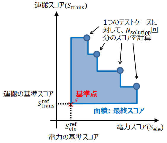
問題文 B
問題 B は問題 A と同様インタラクティブな問題である。 得点(Score)を最大化するように電力をマネジメントしながら効率よく運搬を行うアルゴリズムを作ることが問題 B のタスクである。 Contestantが高得点を獲得するためには、確率的に上下する電力需給に対して、蓄電池を持ちグラフ上を移動する電気自動車(EV)で効率よく運搬を行いながら、蓄電池を持つ頂点(ナノグリッド)の蓄電量を管理することが必要となる。また、電力スコア-運搬スコア平面上で広い領域をカバーできようように、複数の求解で運搬と電力のスコアバランスを調整することも重要である。 作成するプログラムの得点判定の際は、コンテスタント側とジャッジ側が以下で示す流れに沿って処理を行う。
| 繰り返し処理 | コンテスタント | ジャッジ |
|---|---|---|
| 求解回数 N_{\mathrm{solution}} を出力 | ||
| グラフ G を出力 | ||
| 電力需給の情報を出力 | ||
| ナノグリッドの情報を出力 | ||
| EVの情報を出力 | ||
| 運搬の情報を出力 | ||
| スコアの情報を出力 | ||
| 繰り返し処理(ターン)の回数 T_\mathrm{max} を出力 | ||
| for i=1,...,N_{\mathrm{solution}} do for t=0,...,T_\mathrm{max}-1 do |
- | - |
| 時刻 t におけるEVとナノグリッドの状態 \mathrm{info}_t を出力 | ||
| 各EVに対して制御コマンドを出力 | ||
| end for | ||
| 時刻 t=T_\mathrm{max} におけるEVとナノグリッドの状態 \mathrm{info}_t を出力 | ||
| 運搬スコア S_{\mathrm{trans}} と電力スコア S_{\mathrm{ele}} を出力 | ||
| end for |
ジャッジによる求解回数、グラフ、電力需給、ナノグリッド、EV、運搬、スコア、ターン数に関する情報は、はじめに1回だけ出力される。本問題では、0 \leq t \lt T_\mathrm{max} の試行を N_{\mathrm{solution}} 回繰り返すことに注意せよ。各試行で 0 \leq t \lt T_\mathrm{max} を満たす整数 t において、表で示した順番通りに毎回行われる。なお、時刻 t=T_\mathrm{max} における \mathrm{info}_t 及びスコアは必ずコンテスタント側で読み出す必要がある(読み出さない場合TLEになる可能性がある)。
入出力形式1
はじめに、求解回数、グラフ G、電力需給の情報、ナノグリッドの情報、EVの情報、運搬の情報、スコアの情報およびターン数が、以下の形式によりジャッジから標準入力に与えられる。なお、求解回数 2 回目以降の開始時は(下記条件は 1 回目と共通のため)与えられないことに注意せよ。
N_{\mathrm{solution}}
|V| |E|
u_1 v_1 d_1
:
u_{|E|} v_{|E|} d_{|E|}
\mathrm{DayType}
N_\mathrm{div} N_\mathrm{pattern} \sigma^{2}_{\mathrm{ele}} p_{\mathrm{event}} \Delta_{\mathrm{event}}
\mathrm{pw}_{1,1}^{\mathrm{predict}} \mathrm{pw}_{1,2}^{\mathrm{predict}} ... \mathrm{pw}_{1,N_\mathrm{div}}^{\mathrm{predict}}
:
\mathrm{pw}_{N_\mathrm{pattern},1}^{\mathrm{predict}} \mathrm{pw}_{N_\mathrm{pattern},2}^{\mathrm{predict}} ... \mathrm{pw}_{N_\mathrm{pattern},N_\mathrm{div}}^{\mathrm{predict}}
N_\mathrm{grid} C_{\mathrm{init}}^{\mathrm{grid}} C_{\mathrm{max}}^{\mathrm{grid}} V_{\max}^{\mathrm{grid}}
x_1 \mathrm{pattern}_1
:
x_{N_\mathrm{grid}} \mathrm{pattern}_{N_\mathrm{grid}}
N_\mathrm{EV} C_{\mathrm{init}}^{\mathrm{EV}} C_{\mathrm{max}}^{\mathrm{EV}} V_{\max}^{\mathrm{EV}} N_{\max}^{\mathrm{trans}} \Delta_{\mathrm{move}}^{\mathrm{EV}}
\mathrm{pos}_1
:
\mathrm{pos}_{N_\mathrm{EV}}
p_{\mathrm{trans}}^{\mathrm{const}} T_\mathrm{last}
P^{\mathrm{trans}} \gamma S_{\mathrm{ele}}^{\mathrm{ref}} S_{\mathrm{trans}}^{\mathrm{ref}}
T_\mathrm{max}
- 1 行目の N_{\mathrm{solution}} はスコア計算のための求解回数である。
- 続く 1 行で、 |V| はグラフの頂点数、|E| はグラフの辺数が与えられる。
- 続く |E| 行で、グラフの辺が与えられる。 |E| 行のうち i 行目は、頂点 u_{i} と v_{i} の間に距離 d_i の辺が存在することを表す。
- 続く 1 行で、天候タイプ \mathrm{DayType} が与えられる。\mathrm{DayType} は 0: 晴(ゲリラ豪雨無し)、1: 晴(ゲリラ豪雨有り)、2: 雨(想定外の晴れ無し)、3: 雨(想定外の晴れ有り)のいずれかが与えられる。
- 続く 1 行で、予測電力需給が一定値となる区間の数 N_\mathrm{div} と予測電力需給のパターン数 N_\mathrm{pattern} と電力需給の分散 \sigma^{2}_{\mathrm{ele}} とゲリラ豪雨もしくは想定外の晴れの発生確率 p_{\mathrm{event}} (天候タイプが 0 もしくは 2 の場合は 0.0 となる)とゲリラ豪雨もしくは想定外の晴れ発生時の電力需給の変化量 \Delta_{\mathrm{event}} が与えられる。
- 続く N_\mathrm{pattern} 行で各パターンの予測電力需給の値が与えられる。i 行目の j 番目の数値 \mathrm{pw}_{i,j}^{\mathrm{predict}} は、予測電力需給パターン i における時間区間 j 番目の予測電力需給の値を表す。
- 続く 1 行で、ナノグリッドの個数 N_\mathrm{grid} とナノグリッドの時刻 0 での蓄電量 C_{\mathrm{init}}^{\mathrm{grid}} と最大蓄電量 C_{\mathrm{max}}^{\mathrm{grid}} と蓄電池の上限充放電速度 V_{\max}^{\mathrm{grid}} が与えられる。
- 続く N_\mathrm{grid} 行でナノグリッドの情報が与えられる。N_\mathrm{grid} 行のうち i 行目は、頂点 x_i 上に、予測電力需給パターン \mathrm{pattern}_i のナノグリッドが存在することを表す。
- 続く 1 行で、EVの個数 N_\mathrm{EV} とEVの時刻 0 での蓄電量 C_{\mathrm{init}}^{\mathrm{EV}} と最大蓄電量 C_{\mathrm{max}}^{\mathrm{EV}} と蓄電池の上限充放電速度 V_{\max}^{\mathrm{EV}} と運搬物の積載上限数 N_{\max}^{\mathrm{trans}} と単位距離の移動に必要な電力 \Delta_{\mathrm{move}}^{\mathrm{EV}} が与えられる。
- 続く N_\mathrm{EV} 行で、EVの位置が与えられる。N_\mathrm{EV} 行のうち i 行目は、i 番目のEVが頂点 \mathrm{pos}_i 上にあることを表す。
- 続く 1 行で、各時刻で運搬依頼が発生する確率 p_{\mathrm{trans}}^{\mathrm{const}} と運搬依頼が発生する最終時刻 T_\mathrm{last} が与えられる。
- 続く 1 行で、未完了の運搬に対するペナルティ P^{\mathrm{trans}} と不足電力ペナルティ係数 \gamma と電力の基準スコア S_{\mathrm{ele}}^{\mathrm{ref}} と運搬の基準スコア S_{\mathrm{trans}}^{\mathrm{ref}} が与えられる。
- 続く 1 行で、あなたが行動するターン数 T_{\max} が与えられる。
入出力形式2
各時刻 t に、その時刻におけるEVとナノグリッドの状態 \mathrm{info}_t が、以下の形式によりジャッジから標準入力に与えられる。
x_1 y_1 \mathrm{pw}_{1}^{\mathrm{actual},t-1} \mathrm{pw}_{1}^{\mathrm{excess},t-1} \mathrm{pw}_{1}^{\mathrm{buy},t-1}
:
x_{N_\mathrm{grid}} y_{N_\mathrm{grid}} \mathrm{pw}_{N_\mathrm{grid}}^{\mathrm{actual},t-1} \mathrm{pw}_{N_\mathrm{grid}}^{\mathrm{excess},t-1} \mathrm{pw}_{N_\mathrm{grid}}^{\mathrm{buy},t-1}
\mathrm{carinfo}_1
:
\mathrm{carinfo}_{N_\mathrm{EV}}
N_\mathrm{order}
\mathrm{id}_1 w_1 z_1 \mathrm{state}_1 \mathrm{time}_1
...
\mathrm{id}_{N_\mathrm{order}} w_{N_\mathrm{order}} z_{N_\mathrm{order}} \mathrm{state}_{N_\mathrm{order}} \mathrm{time}_{N_\mathrm{order}}
- 始めの N_\mathrm{grid} 行のうち i 行目は、x_i 上に存在するナノグリッドの蓄電量が y_i であり、前時刻 t-1 における実際の電力需給、余って捨てられた電気の量、電力不足で系統から購入した電気の量がそれぞれ \mathrm{pw}_{i}^{\mathrm{actual},t-1}、\mathrm{pw}_{i}^{\mathrm{excess},t-1}、\mathrm{pw}_{i}^{\mathrm{buy},t-1} であることを表す。ただし t=0 においては、 \mathrm{pw}_{i}^{\mathrm{actual},t-1}、\mathrm{pw}_{i}^{\mathrm{excess},t-1}、\mathrm{pw}_{i}^{\mathrm{buy},t-1} はいずれも 0 が表示されるものとする。
補足: \mathrm{pw}_{i}^{\mathrm{actual},t-1}、\mathrm{pw}_{i}^{\mathrm{excess},t-1}、\mathrm{pw}_{i}^{\mathrm{buy},t-1}は、それぞれ ナノグリッドの蓄電池の充放電処理 "処理1"の \Delta^{\mathrm{grid}}_{\mathrm{gen},t-1}、"処理2"の"速度や上限蓄電量を超えた分の電気"\Delta^{\mathrm{grid}}_{\mathrm{total},t-1} - \min \left\{ V_{\max}^{\mathrm{grid}}, C^{\mathrm{grid}}_{\max}-C^{\mathrm{grid}}_{t-1} \right\}、"処理3"の"電力不足分" - \Delta^{\mathrm{grid}}_{\mathrm{total},t-1} - \min \left\{ V_{\max}^{\mathrm{grid}}, C^{\mathrm{grid}}_{t-1} \right\} に対応する。ただし、前時刻 t-1 でそれぞれ"処理2"、"処理3"が実行されなかった場合、\mathrm{pw}_{i}^{\mathrm{excess},t-1} と \mathrm{pw}_{i}^{\mathrm{buy},t-1} はそれぞれ 0 となる。 - 続く N_\mathrm{EV} 項目はそれぞれ 4 行からなり、そのうち i 項目目の \mathrm{carinfo}_i は i 番目のEVの状態を表す。\mathrm{carinfo}_i はそれぞれ後述の形式で与えられる。
- 続く 1 行は、未配達の注文の個数 N_\mathrm{order} を表す。
- 続く N_\mathrm{order} 行のうち i 行目は、注文 \mathrm{id}_i の出発地点が頂点 w_i、到着地点が頂点 z_i、状態が \mathrm{state}_i、発生時刻が \mathrm{time}_i であることを表す。状態について、\mathrm{state}_i=0 のときは注文 \mathrm{id}_i がいまだどのEVにも積まれていないことを表し、\mathrm{state}_i=1 のときは注文 i がいずれかのEVに積まれているが配達が完了していないことを表す。
また、i 番目のEVの状態を表す \mathrm{carinfo}_i は、以下の形式で与えられる。
\mathrm{charge}_i
u_i v_i \mathrm{dist\_from}\_u_i \mathrm{dist\_to}\_v_i
N_{\mathrm{adj},i} a_{i,1} a_{i,2} \ldots a_{i,N_\mathrm{adj}}
N_{\mathrm{order},i} o_{i,1} o_{i,2} \ldots o_{N_{\mathrm{order}, i}}
- 始めの 1 行目は、 i 番目のEVの蓄電量が \mathrm{charge}_i であることを表す。
- 続く 2 行目は、 i 番目のEVの位置を表す。u_i \ne v_i ならば、i 番目のEVは頂点 u_i と 頂点v_i を結ぶ辺上に存在して頂点 u_i から \mathrm{dist\_from}\_u_i、頂点 v_i から \mathrm{dist\_to}\_v_i の距離にあることを表す。u_i = v_i ならば、i 番目のEVはちょうど頂点 u_i 上にあることを表し、\mathrm{dist\_from}\_u_i と \mathrm{dist\_to}\_v_i は共に 0 が出力される。
- 続く 3 行目は、動作
moveで i 番目のEVがその方向に移動可能な頂点が N_{\mathrm{adj},i} 個存在し、それらが頂点 a_{i,1}、頂点 a_{i,2}、\ldots、頂点 a_{i,N_\mathrm{adj}} であることを表す。 - 続く 4 行目は、i 番目のEVが運搬中である注文が N_{\mathrm{order},i} 個存在し、それらが注文o_{i,1}、注文 o_{i,2}、\ldots、注文 o_{N_{\mathrm{order}, i}} であることを表す。
次に、コンテスタントは、時刻 t (0 \leq t \lt T_{\max}) における各EVの動作 \mathrm{command}_i (1 \leq i \leq N_\mathrm{EV}) を標準出力に出力しなければならない。各動作は改行で区切られなくてはならず、また末尾に改行を出力する必要がある。
\mathrm{command}_{1}
\mathrm{command}_{2}
:
\mathrm{command}_{N_\mathrm{EV}}
ここで、\mathrm{command} は以下の形式でなければならない。
stayを行う場合、stayと 1 行で出力move wを行う場合、move wと 1 行で出力pickup aを行う場合、pickup aと 1 行で出力charge_from_grid\Delta^{\mathrm{grid} \rightarrow \mathrm{EV}}_{\mathrm{charge}} を行う場合、charge_from_grid\Delta^{\mathrm{grid} \rightarrow \mathrm{EV}}_{\mathrm{charge}} と 1 行で出力charge_to_grid\Delta^{\mathrm{EV} \rightarrow \mathrm{grid}}_{\mathrm{charge}} を行う場合、charge_to_grid\Delta^{\mathrm{EV} \rightarrow \mathrm{grid}}_{\mathrm{charge}} と 1 行で出力
それぞれの動作には満たすべき条件が存在する(詳細はEVの"動作"の節を参照のこと)。それらの条件を満たさない場合の動作は未定義である。
入出力形式3
コンテスタントが時刻 t=T_\mathrm{max}-1 における各EVの動作を標準出力に出力したのち、ジャッジから時刻 t=T_\mathrm{max} におけるEVとナノグリッドの状態 \mathrm{info}_t が標準入力に与えられる(\mathrm{info}_t の形式は"入出力形式2"を参照)。引き続いて次の行にジャッジから以下の形式で運搬スコア S_{\mathrm{trans}} と電力スコア S_{\mathrm{ele}} が標準入力に与えられる。
S_{\mathrm{trans}} S_{\mathrm{ele}}
入出力制約
- 入力で与えられる数値のうち"[小数]"と記載されているものは小数で与えられ、その他のものは整数で与えられる。
初期化(入出力形式1)
- N_{\mathrm{solution}} = 5
- |V| = 225
- 1.5 |V| \leq |E| \leq 2 |V|
- 1 \leq u_{i}, v_{i} \leq |V|, u_i \ne v_i (1 \leq i \leq |E|)
- 1 \leq d_i \leq \lceil 2\sqrt{2|V|} \rceil (1 \leq i \leq |E|)
- 与えられるグラフは自己ループ・多重辺が存在せず、連結であることが保証される。
- \mathrm{DayType} \in \left\{ 0, 1, 2, 3 \right\}
- N_\mathrm{div} = 20
- N_\mathrm{pattern} = 3
- \sigma^{2}_{\mathrm{ele}} = 100
- p_{\mathrm{event}} \in \left\{ 0.0, 0.1 \right\} "[小数]"
- \Delta_{\mathrm{event}} = 1000
- -1000 \lt \mathrm{pw}_{i,j}^{\mathrm{predict}} \lt 1000 (1 \leq i \leq N_\mathrm{pattern}, 1 \leq j \leq N_\mathrm{div})
- N_\mathrm{grid} = 20
- C_{\mathrm{init}}^{\mathrm{grid}} = 25000
- C_{\mathrm{max}}^{\mathrm{grid}} = 50000
- V_{\max}^{\mathrm{grid}} = 800
- 1 \leq x_i \leq |V| (i \neq j なら x_i \neq x_j, 1 \leq i \leq N_\mathrm{grid})
- 1 \leq \mathrm{pattern}_i \leq N_\mathrm{pattern} (1 \leq i \leq N_\mathrm{grid})
- N_{\min}^{\mathrm{EV}} = 15
- N_{\max}^{\mathrm{EV}} = 25
- N_{\min}^{\mathrm{EV}} \leq N_\mathrm{EV} \leq N_{\max}^{\mathrm{EV}}
- C_{\mathrm{init}}^{\mathrm{EV}} = 12500
- C_{\mathrm{max}}^{\mathrm{EV}} = 25000
- V_{\max}^{\mathrm{EV}} = 400
- N_{\max}^{\mathrm{trans}} = 4
- \Delta_{\mathrm{move}}^{\mathrm{EV}} = 50
- 1 \leq \mathrm{pos}_i \leq |V| (1 \leq i \leq N_\mathrm{EV})
- p_{\mathrm{trans}}^{\mathrm{const}} = 0.7 "[小数]"
- T_\mathrm{last} = 900
- P^{\mathrm{trans}} = 3000
- \gamma = 2.0 "[小数]"
- S_{\mathrm{ele}}^{\mathrm{ref}} = -1,500,000
- S_{\mathrm{trans}}^{\mathrm{ref}} = -1,900,000
- T_\mathrm{max} = 1000
繰り返し処理(入出力形式2)
- 1 \leq x_i \leq |V| (i \neq j なら x_i \neq x_j, 1 \leq i \leq N_\mathrm{grid})
- 0 \leq y_i \leq C_{\mathrm{max}}^{\mathrm{grid}} (1 \leq i \leq N_\mathrm{grid})
- -10000 \lt \mathrm{pw}_{i}^{\mathrm{actual},j} \lt 10000 (1 \leq i \leq N_\mathrm{grid}, -1 \leq j \leq T_\mathrm{max}-2)
- 0 \leq \mathrm{pw}_{i}^{\mathrm{excess},j} \lt 10000, (1 \leq i \leq N_\mathrm{grid}, -1 \leq j \leq T_\mathrm{max}-2)
- 0 \leq \mathrm{pw}_{i}^{\mathrm{buy},j} \lt 10000, (1 \leq i \leq N_\mathrm{grid}, -1 \leq j \leq T_\mathrm{max}-2)
- 0 \leq \mathrm{charge}_i \leq C_{\mathrm{max}}^{\mathrm{EV}} (1 \leq i \leq N_\mathrm{EV})
- 1 \leq u_i, v_i \leq |V| (1 \leq i \leq N_\mathrm{EV})
- 0 \leq \mathrm{dist\_from}\_u_i \leq \lceil 2\sqrt{2|V|} \rceil (1 \leq i \leq N_\mathrm{EV})
- 0 \leq \mathrm{dist\_to}\_v_i \leq \lceil 2\sqrt{2|V|} \rceil (1 \leq i \leq N_\mathrm{EV})
- 1 \leq N_{\mathrm{adj},i} \leq 5(\mathrm{MaxDegree}) (1 \leq i \leq N_\mathrm{EV})
- 1 \leq a_{i,j} \leq |V| (1 \leq i \leq N_\mathrm{EV}, 1 \leq j \leq N_{\mathrm{adj},i})
- 0 \leq N_{\mathrm{order},i} \leq N_{\max}^{\mathrm{trans}} (1 \leq i \leq N_\mathrm{EV})
- 1 \leq o_{i,j} \leq T_\mathrm{last} (1 \leq i \leq N_\mathrm{EV}, 1 \leq j \leq N_{\mathrm{order},i})
- 0 \leq N_\mathrm{order} \leq T_\mathrm{last}
- 1 \leq \mathrm{id}_i \leq T_\mathrm{last} (1 \leq i \leq N_\mathrm{order})
- 1 \leq w_i \leq |V| (1 \leq i \leq N_\mathrm{order})
- 1 \leq z_i \leq |V| (1 \leq i \leq N_\mathrm{order})
- w_i \ne z_i (1 \leq i \leq N_\mathrm{order})
- \mathrm{state}_i \in \left\{ 0, 1 \right\} (1 \leq i \leq N_\mathrm{order})
- 0 \leq \mathrm{time}_i \leq T_\mathrm{last} (1 \leq i \leq N_\mathrm{order})
スコア(入出力形式3)
- S_{\mathrm{trans}} "[小数]"
- S_{\mathrm{ele}} "[小数]"
入出力例
注意: この例はわかりやすさのために小さなセットで入出力を説明したものである。そのためパラメータの値は"入出力制約"に書かれた値とは異なるが、入出力のフォーマット(入出力形式1,2及び3)とEVの動作、及び"ナノグリッドの蓄電池の充放電処理"に書かれた計算方法は実際と同じである。
| 時刻 | ジャッジ | コンテスタント | 説明 |
|---|---|---|---|
1 4 4 1 2 1 2 3 2 3 4 3 4 1 1 0 2 2 1 0 10 5 -2 -4 4 2 10 20 4 1 1 4 2 2 5 10 2 2 1 2 4 0.5 3 3 0.5 -100 -100 4 |
はじめに、ジャッジ側からデータが与えられる。 1 行目: 求解回数は 1 回である。 2 行目: 無向グラフ G は |V| = 4 個の頂点と |E| = 4 本の辺から構成される。 次の 4 行 (3 - 6 行目) は、グラフの辺に関する情報を表す。 3 行目: 辺 1 は頂点 1 と頂点 2 を結んでおり、長さは 1 である。 4 行目: 辺 2 は頂点 2 と頂点 3 を結んでおり、長さは 2 である。 5 行目: 辺 3 は頂点 3 と頂点 4 を結んでおり、長さは 3 である。 6 行目: 辺 4 は頂点 4 と頂点 1 を結んでおり、長さは 1 である。 7 行目: 天候タイプは 0 "晴(ゲリラ豪雨無し)" である。 8 行目: 予想電力需給が一定の時間区間の数は 2 個、ナノグリッドの需要パターンは 2 個、電力需給のゆらぎの分散は 1 、ゲリラ豪雨の発生確率は 0、ゲリラ豪雨発生時の電力需給の低下量は 10 である。 次の 2 行 (9 - 10 行目) は、予想電力需給に関する情報を表す。 9 行目: 需要パターン 1 のナノグリッドの予想電力需給は 5 (時間区間 1)、-2 (時間区間 2)である。 10 行目: 需要パターン 2 のナノグリッドの予想電力需給は -4 (時間区間 1)、4 (時間区間 2)である。 11 行目: グラフ G の頂点のうちナノグリッドがあるものは N_\mathrm{grid} = 2 個、時刻 t=0 におけるナノグリッドの蓄電量は C_{\mathrm{init}}^{\mathrm{grid}} = 10、最大蓄電量は C_{\mathrm{max}}^{\mathrm{grid}} = 20、上限充放電速度は V_{\max}^{\mathrm{grid}} = 4 である。 12 行目: ナノグリッド 1 は頂点 1 上にあり、需要パターンは 1 である。 13 行目: ナノグリッド 2 は頂点 4 上にあり、需要パターンは 2 である。 14 行目: あなたが動作させることができるEVの台数は N_\mathrm{EV} = 2 台、時刻 t=0 におけるEVの蓄電量は C_{\mathrm{init}}^{\mathrm{EV}} = 5、最大蓄電量は C_{\mathrm{max}}^{\mathrm{EV}} = 10、上限充放電速度は V_{\max}^{\mathrm{EV}} = 2 、同時に 1 台のEVに積載可能な運搬物の上限数は N_{\max}^{\mathrm{trans}} = 2、単位時間のEVの移動で減少する蓄電量は \Delta_{\mathrm{move}}^{\mathrm{EV}} = 1 である。 次の 2 行 (15 - 16 行目) は時刻 t=0 における各EVの位置を表す。 15 行目: EV 1 は時刻 t=0 で頂点 2 上にある。 16 行目: EV 2 は時刻 t=0 で頂点 4 上にある。 17 行目: 各時刻で新しい運搬依頼が発生する確率は p_{\mathrm{trans}}^{\mathrm{const}} = 0.5 であり、新しい運搬依頼が発生する最終時刻は T_\mathrm{last} = 3 である。 18 行目: 最終時刻まで完了しない運搬依頼 1 つあたり、P^{\mathrm{trans}} = 3 点が減点される。ナノグリッドが外部から補充した単位電気量あたりの減点は \gamma = 0.5 点である。電力スコアの基準スコアは S_{\mathrm{ele}}^{\mathrm{ref}} = -100 点であり、運搬スコアの基準スコアは S_{\mathrm{trans}}^{\mathrm{ref}} = -100 点である。 19 行目: あなたが行動するターン数は T_{\max} = 4 である。 |
||
| 0 | 1 10 0 0 0 4 10 0 0 0 5 2 2 0 0 2 1 3 0 5 4 4 0 0 2 1 3 0 1 1 1 4 0 0 |
move 1 charge_from_grid 2 |
次いで、ジャッジ側から時刻 0 でのデータが与えられる。 1 行目: 頂点 1 にあるナノグリッドの時刻 0 での蓄電量は 10 である(時刻 0 の場合、残りの 3 つの値は必ず 0 である)。 2 行目: 頂点 4 にあるナノグリッドの時刻 0 での蓄電量は 10 である(時刻 0 の場合、残りの 3 つの値は必ず 0 である)。 次の 4 行 (3 - 6 行目) は、EV 1 の状態を表す。 3 行目: EV 1 の時刻 0 での蓄電量は 5 である。 4 行目: EV 1 は時刻 0 において頂点 2 上に位置する。 5 行目: EV 1 が `move` コマンドでその方向に向かって移動可能な頂点は N_{\mathrm{adj},1} = 2 個あり、頂点 1 および頂点 3 である。 6 行目: EV 1 が 運搬中である注文は N_{\mathrm{order},i} = 0 個である。 次の 4 行 (7 - 10 行目) は、EV 2 の状態を表す。 7 行目: EV 2 の時刻 0 での蓄電量は 5 である。 8 行目: EV 2 は時刻 0 において頂点 4 上に位置する。 9 行目: EV 2 が `move` コマンドでその方向に向かって移動可能な頂点は N_{\mathrm{adj},2} = 2 個あり、頂点 1 および頂点 3 である。 10 行目: EV 2 が 運搬中である注文は N_{\mathrm{order},i} = 0 個である。 11 行目: 未配達の注文が N_\mathrm{order} = 1 個存在する。 12 行目: 注文 1 は頂点 1 から頂点 4 への配達であり、どのEVにも積まれておらず、時刻 0 に発生したものである。 これに対するコンテスタントの出力は以下のとおりである。 1 行目: EV 1 を頂点 1 の方向へ移動させようとする。EV 1 の充電が 1 消費されるが、蓄電量が 1 以上であったため移動は成功する。頂点 1 から頂点 2 への辺の長さは 1 であるので、時刻 1 に頂点 2 へ移動することが可能である。 2 行目: EV 2 はナノグリッドから 2 だけ充電する。EV 2 はナノグリッド上にあり、充電量はEV 2 の上限充放電速度 2 を超えない。またEV 2 の充電後の蓄電量は最大蓄電量 10 を超えない。したがって動作条件を満たすので、時刻 1 に充電量を 7 に増やすことが可能である。 |
| 1 | 1 14 5 1 0 4 6 -4 0 2 4 1 1 0 0 2 2 4 0 7 4 4 0 0 2 1 3 0 1 1 1 4 0 0 |
pickup 1 charge_from_grid 2 |
次いで、ジャッジ側から時刻 1 でのデータが与えられる。 1 行目: 頂点 1 にあるナノグリッドの時刻 1 での蓄電量は 14 であり、前時刻 t=0 における実際の電力需給、余って捨てられた電気の量、電力不足で系統から購入した電気の量がそれぞれ 5, 1, 0 である(ナノグリッドの上限充放電速度を超える分は捨てられる)。 2 行目: 頂点 4 にあるナノグリッドの時刻 1 での蓄電量は 6 であり、前時刻 t=0 における実際の電力需給、余って捨てられた電気の量、電力不足で系統から購入した電気の量がそれぞれ -4, 0, 2 である。 次の 4 行 (3 - 6 行目) は、EV 1 の状態を表す。 3 行目: EV 1 の時刻 1 での蓄電量は 4 である。 4 行目: EV 1 は時刻 1 において頂点 1 上に位置する。 5 行目: EV 1 が `move` コマンドでその方向に向かって移動可能な頂点は N_{\mathrm{adj},1} = 2 個あり、頂点 2 および頂点 4 である。 6 行目: EV 1 が 運搬中である注文は N_{\mathrm{order},i} = 0 個である。 次の 4 行 (7 - 10 行目) は、EV 2 の状態を表す。 7 行目: EV 2 の時刻 1 での蓄電量は 7 である。 8 行目: EV 2 は時刻 1 において頂点 4 上に位置する。 9 行目: EV 2 が `move` コマンドでその方向に向かって移動可能な頂点は N_{\mathrm{adj},2} = 2 個あり、頂点 1 および頂点 3 である。 10 行目: EV 2 が 運搬中である注文は N_{\mathrm{order},i} = 0 個である。 11 行目: 未配達の注文が N_\mathrm{order} = 1 個存在する。 12 行目: 注文 1 は頂点 1 から頂点 4 への配達であり、どのEVにも積まれておらず、時刻 0 に発生したものである。 これに対するコンテスタントの出力は以下のとおりである。 1 行目: 頂点 1 に位置するEV 1 に注文 1 を積む。充電は消費されない。 2 行目: EV 2 はナノグリッドから 2 だけ充電する。EV 2 はナノグリッド上にあり、充電量はEV 2 の上限充放電速度 2 を超えない。またEV 2 の充電後の蓄電量は最大蓄電量 10 を超えない。したがって動作条件を満たすので、時刻 2 に充電量を 9 に増やすことが可能である。 |
| 2 | 1 18 5 1 0 4 2 -4 0 2 4 1 1 0 0 2 2 4 1 1 9 4 4 0 0 2 1 3 0 2 1 1 4 1 0 2 4 1 0 2 |
move 4 pickup 2 |
次いで、ジャッジ側から時刻 2 でのデータが与えられる。 1 行目: 頂点 1 にあるナノグリッドの時刻 2 での蓄電量は 18 であり、前時刻 t=1 における実際の電力需給、余って捨てられた電気の量、電力不足で系統から購入した電気の量がそれぞれ 5, 1, 0 である。 2 行目: 頂点 4 にあるナノグリッドの時刻 2 での蓄電量は 2 であり、前時刻 t=1 における実際の電力需給、余って捨てられた電気の量、電力不足で系統から購入した電気の量がそれぞれ -4, 0, 2 である。 次の 4 行 (3 - 6 行目) は、EV 1 の状態を表す。 3 行目: EV 1 の時刻 2 での蓄電量は 4 である。 4 行目: EV 1 は時刻 2 において頂点 1 上に位置する。 5 行目: EV 1 が `move` コマンドでその方向に向かって移動可能な頂点は N_{\mathrm{adj},1} = 2 個あり、頂点 2 および頂点 4 である。 6 行目: EV 1 が 運搬中である注文は N_{\mathrm{order},i} = 1 個であり、注文 1 を運搬中である。 次の 4 行 (7 - 10 行目) は、EV 2 の状態を表す。 7 行目: EV 2 の時刻 2 での蓄電量は 9 である。 8 行目: EV 2 は時刻 2 において頂点 4 上に位置する。 9 行目: EV 2 が `move` コマンドでその方向に向かって移動可能な頂点は N_{\mathrm{adj},2} = 2 個あり、頂点 1 および頂点 3 である。 10 行目: EV 2 が 運搬中である注文は N_{\mathrm{order},i} = 0 個である。 11 行目: 未配達の注文が N_\mathrm{order} = 2 個存在する。 12 行目: 注文 1 は頂点 1 から頂点 4 への配達であり、いずれかのEV(この場合はEV 1)に積まれており、時刻 0 に発生したものである。 13 行目: 注文 2 は頂点 4 から頂点 1 への配達であり、どのEVにも積まれておらず、時刻 2 に発生したものである。 これに対するコンテスタントの出力は以下のとおりである。 1 行目: EV 1 を頂点 4 の方向へ移動させようとする。EV 1 の充電が 1 消費されるが、蓄電量が 1 以上であったため移動は成功する。頂点 1 から頂点 4 への辺の長さは 1 であるので、時刻 3 に頂点 4 へ移動することが可能である。 2 行目: 頂点 4 に位置するEV 2 に注文 2 を積む。充電は消費されない。 |
| 3 | 1 17 -1 0 0 4 6 4 0 0 3 4 4 0 0 2 1 3 0 9 4 4 0 0 2 1 3 1 2 1 2 4 1 1 2 |
stay move 1 |
次いで、ジャッジ側から時刻 3 でのデータが与えられる。 1 行目: 頂点 1 にあるナノグリッドの時刻 3 での蓄電量は 17 であり、前時刻 t=2 における実際の電力需給、余って捨てられた電気の量、電力不足で系統から購入した電気の量がそれぞれ -1, 0, 0 である(電力需給の予測値は -2 だがゆらぎにより実際の値は -1 となった)。 2 行目: 頂点 4 にあるナノグリッドの時刻 3 での蓄電量は 6 であり、前時刻 t=2 における実際の電力需給、余って捨てられた電気の量、電力不足で系統から購入した電気の量がそれぞれ 4, 0, 0 である。 次の 4 行 (3 - 6 行目) は、EV 1 の状態を表す。 3 行目: EV 1 の時刻 3 での蓄電量は 3 である。 4 行目: EV 1 は時刻 3 において頂点 4 上に位置する。 5 行目: EV 1 が `move` コマンドでその方向に向かって移動可能な頂点は N_{\mathrm{adj},1} = 2 個あり、頂点 1 および頂点 3 である。 6 行目: EV 1 が 運搬中である注文は N_{\mathrm{order},i} = 0 個である。前時刻まで積載していた注文 1 は目的地頂点 4 に到達したため、降ろされた。 次の 4 行 (7 - 10 行目) は、EV 2 の状態を表す。 7 行目: EV 2 の時刻 3 での蓄電量は 9 である。 8 行目: EV 2 は時刻 3 において頂点 4 上に位置する。 9 行目: EV 2 が `move` コマンドでその方向に向かって移動可能な頂点は N_{\mathrm{adj},2} = 2 個あり、頂点 1 および頂点 3 である。 10 行目: EV 2 が 運搬中である注文は N_{\mathrm{order},i} = 1 個であり、注文 2 を運搬中である。 11 行目: 未配達の注文が N_\mathrm{order} = 1 個存在する。 12 行目: 注文 2 は頂点 4 から頂点 1 への配達であり、いずれかのEV(この場合はEV 2)に積まれており、時刻 2 に発生したものである。 これに対するコンテスタントの出力は以下のとおりである。 1 行目: EV 1 はその場にとどまる 2 行目: EV 2 を頂点 1 の方向へ移動させようとする。EV 1 の充電が 1 消費されるが、蓄電量が 1 以上であったため移動は成功する。頂点 4 から頂点 1 への辺の長さは 1 であるので、時刻 4 に頂点 1 へ移動することが可能である。また、積んでいる注文 2 の到着地点は頂点 1 であるので、その際に注文 2 が完了する。 |
| 4 | 1 15 -2 0 0 4 10 5 1 0 3 4 4 0 0 2 1 3 0 8 1 1 0 0 2 2 4 0 0 3.0 34.0 |
最後に、ジャッジ側から時刻 4 でのデータが与えられる。 1 行目: 頂点 1 にあるナノグリッドの時刻 4 での蓄電量は 15 であり、前時刻 t=3 における実際の電力需給、余って捨てられた電気の量、電力不足で系統から購入した電気の量がそれぞれ -2, 0, 0 である。 2 行目: 頂点 4 にあるナノグリッドの時刻 4 での蓄電量は 10 であり、前時刻 t=3 における実際の電力需給、余って捨てられた電気の量、電力不足で系統から購入した電気の量がそれぞれ 5, 1, 0 である(電力需給の予測値は 4 だがゆらぎにより実際の値は 5 となった)。 次の 4 行 (3 - 6 行目) は、EV 1 の状態を表す。 3 行目: EV 1 の時刻 4 での蓄電量は 3 である。 4 行目: EV 1 は時刻 4 において頂点 4 上に位置する。 5 行目: EV 1 が `move` コマンドでその方向に向かって移動可能な頂点は N_{\mathrm{adj},1} = 2 個あり、頂点 1 および頂点 3 である。 6 行目: EV 1 が 運搬中である注文は N_{\mathrm{order},i} = 0 個である。 次の 4 行 (7 - 10 行目) は、EV 2 の状態を表す。 7 行目: EV 2 の時刻 4 での蓄電量は 8 である。 8 行目: EV 2 は時刻 4 において頂点 1 上に位置する。 9 行目: EV 2 が `move` コマンドでその方向に向かって移動可能な頂点は N_{\mathrm{adj},2} = 2 個あり、頂点 2 および頂点 4 である。 10 行目: EV 2 が 運搬中である注文は N_{\mathrm{order},i} = 0 個である。前時刻まで積載していた注文 2 は目的地頂点 1 に到達したため、降ろされた。 11 行目: 未配達の注文が N_\mathrm{order} = 0 個存在する。 次の 1 行 (12 行目) は、運搬スコア及び電力スコアを表す。 12 行目: 運搬スコアは 3となり、電力スコアは34.0となる。 計算方法: 運搬は 2 つ発生し、それぞれの待ち時間 3、2 であり、未運搬は無いため、運搬スコアは (4-3)+(4-2)-0=3.0 と計算される。電力は、EV 2 台の最終時刻の蓄電量がそれぞれ 3、8 であり、ナノグリッド 2 箇所の最終時刻の蓄電量がそれぞれ 15、10 であるため、総残電力は 36 となる。また、系統からの購入電力量が合計で 4 (頂点 4 のナノグリッドが時刻 0 と 1 でそれぞれ 2 ずつ購入)なので、電力スコアは 36-0.5 \times 4=34.0 と計算される。 |
サンプルコード B
問題Bのツールキット一式はここからダウンロードできます。
このツールキットを用いて、手元の環境で入力サンプル(テストケース)の生成や、ジャッジの実行が可能です。また、ビギナー向けのサンプルコードも用意しています。
小さなバグが見つかったため、ツールキットを修正しました(12/18)。
windowsでも利用可能なツールキットを公開しました(Cygwin,WSLで動作確認済)。合わせて英語版のREADME(short ver.)も追加しました。また、辺数の制約に関するバグの修正をしています。(12/18)
英語版のREADME(full ver.)を公開しました。また、日本語版のREADMEの細かな誤りを修正しました。(12/21)
ジャッジシステムの修正(python等投稿対応)に合わせてツールキットを修正しました。また、Pythonのサンプルコードも同梱しました。使い方はREADMEを御覧ください。(1/6)
ツールキットを修正しました(DEBUG_LEVELに関する修正など)。また、サンプルコードの微修正も行いました。(1/12)
- 入力サンプルジェネレータ
- テスター
- ビキナー向けのサンプルコード
Table of contents
Problem Summary
Time Schedules and Spatial Structures
Constitution of a Nanogrid
Energy Balance
Order Processing
EV Operation
Charge/Discharge to the Battery of a Nanogrid
Scoring
Problem B
Input and Output Format 1
Input and Output Format 2
Input and Output Format 3
Constraints for Input and Output
Example of Inputs and Outputs
Sample Code B
Problem Summary
In this problem, you operate multiple electric vehicles (EVs) so that you can transport customers and goods from one place to another place efficiently while protecting distributed nanogrids from overloading the electrical supply to EVs and providing additional power from EVs if there is a power shortage in the nanogrids. Since EVs consume electricity proportional to their distances traveled, they need to charge from nanogrids if necessary. Each nanogrid is equipped with a battery, a photovoltaic (PV) power system and a fuel engine. Power generation, consumption and charge/discharge to EVs occur in each nanogrid and their time-varying imbalance is compensated by charge/discharge from the battery and electrical supply from outside.

The toolkit, which can be downloaded from the bottom of this page, contains a sample of contestant code in which input/output such as reading data from the judge code has already been implemented. Also, regarding the operation of EV, "all stay", "random walk", and "multiple transportation" have been implemented as examples. When implementing a new algorithm, the sample is designed so that you can focus on describing the operation of EV by inheriting the strategy class. (See README.md for details.) You can use the sample when submitting your code.
Time Schedules and Spatial Structures
- Time Schedules: The total time length of each test case corresponds physically to one business day. The time variable t is supposed to be integer valued ranging from 0 to T_{max}. For each test case, one of the four different one day weather patterns is randomly assigned and the weather pattern affects the resulting time series of difference between generated and consumed powers (energy balance). In the beginning of each test case, each contestant gets a whole time series of predicted energy balance and, for each time t, each contestant gets the charged capacity of the battery for each nanogrid, the set of orders assigned so far, and the following values in the previous step: actual energy balance, excess amount of power discarded, and power supplied from the outside. Based on the information, each contestant is asked to decide how to operate multiple EVs in the next step for each time t.
- Spatial Structures: Let G = (V, E) be a simple and undirected graph with the vertex set V and the edge set E, which represents a road network on which EV transportation and EV charge/discharge occur. Nanogrids are located on some of the vertices. An edge represents the road connecting its two endpoints and has a positive integer weight corresponding to the road distance. The graph is generated by the algorithm below.
Algorithm to generate the graph G
For all test cases, the graph G = (V, E) is generated by the following algorithm.- Input:|V|, |E|, \mathrm{MaxDegree}=5
- Algorithm to generate the vertices:
- Find the maximum non-negative integer R such that |V| = R^{2} + r holds for a non-negative integer r.
- For each lattice point satisfying 0 \leq x, y < R in the xy plane, plot a point (x, y).
- Shift each point such as (x, y) \leftarrow (x + dx, y + dy) where dx and dy are random numbers sampled uniformly from the interval [0, 1].
- Remaining r points are plotted at (x', y') where x' and y' are random numbers sampled uniformly from the interval [0, R].
- Assign a separate ID ranging from 1 to |V| to each point and identify each point to the vertex having the assigned ID.
- Algorithm to generate the |V|-1 edges and their weights to guarantee the connectivity of the resulting graph:
- Generate the complete graph G_{\text{comp}} with the vertex set V. For each pair of vertices u, v \in V, assign the Euclidean distance between the points corresponding to u and v to the edge weight W_{u,v}.
- Generate the minimum spanning tree for G_{\text{comp}} and add |V|-1 edges in the minimum spanning tree to the graph G. For each edge \left\{ u, v \right\}, assign \lceil 2 \times W_{u, v} \rceil to the edge weight d_{u,v}.
- Algorithm to generate the remaining |E|-(|V|-1) edges and their weights:
- Remaining |E|-(|V|-1) edges are generated by the following algorithm.
- Update \mathrm{cost}(u,v) based on the algorithm below.
- Find the pair of vertices u and v minimizing \mathrm{cost(u,v)} among all the pairs of vertices not connected by the edges added to the graph G so far and add the edge \left\{ u, v \right\} connecting the pair to the graph G.
- Assign \lceil 2 \times W_{u, v} \rceil to the edge weight d_{u,v}.
-
Here \mathrm{cost}(u,v) is basically determined by the Euclidean distance between the points corresponding to u and v but is biased so that a pair of vertices u and v one of whose degree is small and a pair of vertices lining up vertically and horizontally rather than diagonally are likely to be selected. Due to the bias, the resulting graph is expected to be close to a planer graph. In what follows, we show the algorithm to compute \mathrm{cost}(u,v).
- Compute the degree \mathrm{degree}(u) of the vertex u\in V. The degree \mathrm{degree}(u) of the vertex u\in V is defined by the number of edges incident to the vertex.
- Assign a color to each vertex u\in V as follows: Colors of the first added R^{2} vertices are determined based on their original lattice points (x,y) based on the rule below. Colors of the remaining r vertices are randomly assigned to be 0 or 1.
- If x+y is even : \mathrm{color}(u) = 0
- If x+y is odd : \mathrm{color}(u) = 1
- Bias factor f(u,v) is determined by the following rule:
- If \mathrm{color}(u) = \mathrm{color}(v) : \mathrm{f}(u,v) = 5
- If \mathrm{color}(u) \neq \mathrm{color}(v) : \mathrm{f}(u,v) = 1
- Bias factor g(u) is determined by the following rule:
- If \mathrm{degree}(u) \lt \mathrm{MaxDegree} : g(u)=1
- If \mathrm{degree}(u) \geq \mathrm{MaxDegree} : g(u)=\infty
- Compute \mathrm{cost}(u,v) as follows:
- \mathrm{cost}(u,v) = W_{u,v}\times \mathrm{degree}(u) \times \mathrm{degree}(v) \times f(u,v) \times g(u) \times g(v).
- Remaining |E|-(|V|-1) edges are generated by the following algorithm.
- Algorithm to select vertices where nanogrids are located :
- Uniformly and randomly select N_{\mathrm{grid}} distinct vertices from V and locate a nanogrid on each selected vertex. The set of the vertices on which nanogrids are located is denoted as V_{\mathrm{grid}}.
Constitution of a Nanogrid
Each nanogrid consists of a battery, a photovoltaic (PV) power system, a fuel engine, charging/discharging stations for EVs and power consumers and has the following attributes.
-
Vertex ID: ID of the vertex u on which the nanogrid is located where u \in V_{\mathrm{grid}} (V_{\mathrm{grid}}: the set of vertices on which nanogrids are located (See "Algorithm to generate the graph G".) )
-
Charged Capacity: The charged capacity of the battery in the nanogrid. Its initial value is C_{\mathrm{init}}^{\mathrm{grid}} and its maximum value is C_{\mathrm{max}}^{\mathrm{grid}}, which are the same for all the nanogrids. For each time t, the charged capacity changes by the difference between generated and consumed powers (energy balance) and it also changes by the difference between discharged and charged electricity to EVs (For the detail, see Charge/Discharge to the Battery of a Nanogrid .). If the resulting charged capacity exceeds C_{\mathrm{max}}^{\mathrm{grid}} at the time t, the charged capacity is set to C_{\mathrm{max}}^{\mathrm{grid}} at the time t+1 and the excess amount is discarded. Instead, if the resulting capacity is negative at the time t, the shortage is supplied from outside and the charged capacity is set to 0 at the time t+1. If the latter is the case, the score is deducted in proportion to the amount of shortage (For the detail, see Scoring.)
-
Energy Balance: Difference between generated and consumed powers except for those for charging/discharging EVs for each time t. Its predicted value for each time t is provided to contestants in the beginning of each test case. Its actual value is sums of the predicted value and random value caused by stochastic fluctuation of the environment and sudden weather changes like downpour and sudden clear sky (For the detail, see Energy Balance below.)
-
Maximum charging/discharging speed: The maximum speed of charging/discharging to the battery V_{\max}^{\mathrm{grid}}, which is the same for all the nanogrids.
Energy Balance
Difference between generated and consumed powers except for those for charging/discharging EVs for each time t.
-
Pattern of the time series of the energy balance: For each test case, one of the four different one day weather patterns, i.e., sunny with/without downpour and rainy with/without sudden clear sky is randomly assigned and is informed to each contestant in the beginning of the test case. For each nanogrid, one of the N_{\mathrm{pattern}} different expected demand patterns is randomly assigned and is informed to each contestant in the beginning of each test case. A whole time series of predicted energy balance is provided to each contestant in the beginning of each test case. The amount of generated powers from the PV power system depends on the weather pattern and thus the sums of the predicted values of energy balance in one business day is largest for the weather pattern, sunny without downpour, and is smallest for the weather pattern, rainy without sudden clear sky.
-
The time series of the energy balance: The time series of the energy balance is sums of predicted one and stochastic fluctuation \delta and the variation due to downpour and sudden clear sky.
- The total time interval 0 \leq t < T_{\max} is divided into N_{\mathrm{div}} subintervals of equal length and predicted value of the energy balance is constant for each subdivided interval.
- For each time t, \delta is sampled from the normal distribution with the mean 0 and the variance \sigma^{2}_{\mathrm{ele}}. The variance is informed to each contestant in the beginning of each test case but the value \delta is not informed to each contestant in advance.
- Downpour: If the weather pattern is 1 (sunny with downpour), downpour occurs with a probability p_{\mathrm{event}} for each of N_{\mathrm{div}} subintervals. The probability is constant and independent for each subinterval. If the downpour occurs, the energy balance is subtracted by \Delta_{\mathrm{event}} for 15 percent of the nanogrids randomly and independently chosen for each subinterval because generated power from a photovoltaic (PV) power system decreases.
- Sudden clear sky: If the weather pattern is 3 (rainy with sudden clear sky), sudden clear sky occurs with the probability p_{\mathrm{event}} for each of the N_{\mathrm{div}} subintervals. If the sudden clear sky occurs, the energy balance is added by \Delta_{\mathrm{event}} for 15 percent of the nanogrids randomly and independently chosen for each subinterval because generated power from a photovoltaic (PV) power system increases.
In case of the weather patterns 1 and 3, the timing for downpour or sudden clear sky is not informed to each contestant in advance.
Order Processing
An order to transport goods from one vertex u \in V to another vertex v \in V is randomly generated based on the algorithm below for each time t and each contestant is asked to process the order by picking it up at the vertex u and delivering it to the vertex v by operating EVs. In what follows, we call u a starting vertex and v a destination vertex.
-
Attributes for order:
- Order ID (1,...)
- Load time (0 \leq t \leq T_{\mathrm{last}}(<T_{\max}))
- Starting vertex (1,...,|V|)
- Destination vertex (1,...,|V|)
- State (0 if none of the EVs picks the order up and 1 if one of the EVs picked it up but it is not yet delivered.)
-
Algorithm to generate orders: For each time t satisfying 0 \leq t \leq T_{\mathrm{last}}(<T_{\max}), a new order is randomly generated with the probability p_{\mathrm{trans}}^{\mathrm{const}}. Its starting vertex is randomly selected from the vertex set V and its destination vertex is randomly selected from all the vertices except for the starting vertex.
-
Penalty for outstanding orders: For each outstanding order by t=T_{\max}, a penalty P^{\mathrm{trans}} is subtracted from the score for transportation (For the details, see Scoring.).
EV Operation
Each contestant is asked to operate multiple electric vehicles (EVs) to transport customers and goods from one place to another place efficiently while protecting distributed nanogrids from overloading the electrical supply to EVs and providing additional power from EVs if there is a power shortage in the nanogrids.
-
Number of EVs: The number of EVs N^{\mathrm{EV}} is uniformly randomly selected from the interval [N_{\min}^{\mathrm{EV}}, N_{\max}^{\mathrm{EV}}] and is informed to each contestant in the beginning of each test case.
-
Initial Position of EVs: In the beginning of each test case, N^{\mathrm{EV}} vertices are selected randomly and one EV is placed on each selected vertex.
-
Attributes for EV: Each EV has the following attributes:
- ID (0, 1,... , N^{\mathrm{EV}}-1)
- Charged capacity: C^{\mathrm{EV}}_{t} non-negative integer valued, initialized to C^{\mathrm{EV}}_{t=0}, and has the upper limit C^{\mathrm{EV}}_{\max} common for all the EVs
- Present location: either on a vertex or on an edge
- Order IDs located on each EV: The upper limit of number of orders located on each EV is N_{\max}^{\mathrm{trans}}, which is common for all the EVs.
- Maximum charging/discharging speed: V_{\max}^{\mathrm{EV}}, which is common for all the EVs.
-
Operation for EVs: For each time t, each contestant chooses one of the operations below for each EV:
stay: Let the EV stay in the same place. In this case, the EV does not consume electricity, i.e., C^{\mathrm{EV}}_{t+1}-C^{\mathrm{EV}}_{t}=0.-
move w: Let the EV move forward to the vertex w \in V by the distance 1. The charged capacity of the EV in the next step decreases by \Delta^{\mathrm{EV}}_{\mathrm{move}} unless the resulting charged capacity is negative. If that is the case, the operation is rejected, the EV stays at the same position and its charged capacity does not change if the following conditions are satisfied.- Suppose the operation
move wis selected. Then, each contestant getsWA(Wrong Answer) if one of the conditions below are violated.- w \in V
- Supposing the present position of the EV is on u \in V, \left\{ u, w \right\} \in E holds.
- Supposing the present position of the EV is on \left\{ u, v \right\}, w = u or w = v holds.
- Suppose the operation
-
pickup a: Pick the order of ID a by EV. In this operation EV does not consume electricity (An order is automatically delivered when an EV carrying the order arrives at the destination vertex of the order).- Suppose the operation
pickup ais selected. Then, each contestant getsWA(Wrong Answer) if one of the conditions below are violated.- EV is on u \in V
- There is an order of ID a that has the starting vertex u and state 0.
- The number of orders put on the EV is less than N_{\max}^{\mathrm{trans}}.
- Suppose the operation
-
charge_from_grid\Delta^{\mathrm{grid} \rightarrow \mathrm{EV}}_{\mathrm{charge}}: Charge the EV by \Delta^{\mathrm{grid} \rightarrow \mathrm{EV}}_{\mathrm{charge}}. The charged capacity of the EV in the next step C^{\mathrm{EV}}_{t+1} becomes C^{\mathrm{EV}}_{t+1} \leftarrow C^{\mathrm{EV}}_{t} + \Delta^{\mathrm{grid} \rightarrow \mathrm{EV}}_{\mathrm{charge},t}. It is possible to charge multiple EVs from a single nanogrid.- Suppose the operation
charge_from_gridis selected with \Delta^{\mathrm{grid} \rightarrow \mathrm{EV}}_{\mathrm{charge}}. Then, each contestant getsWA(Wrong Answer) if one of the conditions below is violated.- EV is on a vertex where a nanogrid is located u \in V_{\mathrm{grid}}.
- \Delta^{\mathrm{grid} \rightarrow \mathrm{EV}}_{\mathrm{charge}} is a natural number.
- Charged amount for each EV does not exceed the maximum charge/discharge speed: \Delta^{\mathrm{grid} \rightarrow \mathrm{EV}}_{\mathrm{charge}} \leq V_{\max}^{\mathrm{EV}}
- The resulting charged capacity for each EV does not exceed the upper limit C^{\mathrm{EV}}_{\max}: C^{\mathrm{EV}}_{t} + \Delta^{\mathrm{grid} \rightarrow \mathrm{EV}}_{\mathrm{charge}} \leq C^{\mathrm{EV}}_{\max}
- Suppose the operation
-
charge_to_grid\Delta^{\mathrm{EV} \rightarrow \mathrm{grid}}_{\mathrm{charge}}: Charge a nanogrid from the EV by \Delta^{\mathrm{EV} \rightarrow \mathrm{grid}}_{\mathrm{charge}}. The charged capacity of the EV in the next step C^{\mathrm{EV}}_{t+1} becomes C^{\mathrm{EV}}_{t+1} \leftarrow C^{\mathrm{EV}}_{t} - \Delta^{\mathrm{EV} \rightarrow \mathrm{grid}}_{\mathrm{charge},t}. It is possible to charge a nanogrid from multiple EVs. It is also possible to charge EVs from a nanogrid and charge the nanogrid from other EVs simultaneously.- Suppose the operation
charge_to_gridis selected with \Delta^{\mathrm{EV} \rightarrow \mathrm{grid}}_{\mathrm{charge}}. Then, each contestant getsWA(Wrong Answer) if one of the conditions below is violated.- EV is on a vertex where a nanogrid is located u \in V_{\mathrm{grid}}.
- \Delta^{\mathrm{EV} \rightarrow \mathrm{grid}}_{\mathrm{charge}} is a natural number.
- Charged amount for each EV does not exceed the maximum charge/discharge speed: \Delta^{\mathrm{EV} \rightarrow \mathrm{grid}}_{\mathrm{charge}} \leq V_{\max}^{\mathrm{EV}}
- The resulting charged capacity for each EV is not negative: C^{\mathrm{EV}}_{t} - \Delta^{\mathrm{EV} \rightarrow \mathrm{grid}}_{\mathrm{charge}} \geq 0
- Suppose the operation
Charge/Discharge to the Battery of a Nanogrid
For each nanogrid, the charged capacity of the battery varies in time depending on the difference between generated and consumed powers and the amount of charge/discharge to EVs. For each time t, sums of the difference between generated and consumed powers and gross difference between charged/discharged amounts to EVs from the nanogrid correspond to power excess or shortage in the nanogrid. If the power excess occurs, the battery is charged by the amount provided that the power excess does not exceed the maximum charge speed of the battery and the resulting charged capacity of the battery does not exceed its upper limit. If the power excess exceeds the maximum charge speed of the battery, the excess amount is discarded and the battery is charged by the maximum charge speed. If the resulting charged capacity of the battery exceeds its upper limit, the charged capacity is set to the upper limit at the next step and the excess amount is discarded. If the power shortage occurs instead, the power shortage is compensated by discharging the battery provided that the power shortage does not fall below the maximum discharge speed of the battery and the resulting charged capacity of the battery is not negative. If the power shortage falls below the maximum discharge speed of the battery, the power shortage is covered by discharging the battery by the maximum discharge speed and by power supplied from the outside. If the resulting charged capacity of the battery is negative, the charged capacity of the battery is set to zero in the next step and shortage is supplied from the outside. In all the cases, each EV is charged or discharged by the amount prescribed by each contestant.
Algorithm to determine an amount of charge/discharge to the battery in the next step consists of the following 4 steps.
-
Step 1: Compute the power excess or shortage in each nanogrid at time t \Delta^{\mathrm{grid}}_{\mathrm{total}}.
\Delta^{\mathrm{grid}}_{\mathrm{total}} = \Delta^{\mathrm{grid}}_{\mathrm{gen},t} - \sum_{i \in \mathrm{all EV}} \Delta^{\mathrm{grid} \rightarrow \mathrm{EV}i}_{\mathrm{charge},t} + \sum_{i \in \mathrm{all EV}} \Delta^{\mathrm{EV}i \rightarrow \mathrm{grid}}_{\mathrm{charge},t}
Here, each variable is defined as follows.- \Delta^{\mathrm{grid}}_{\mathrm{gen},t}: the difference between generated and consumed powers at the nanogrid at the time t, which is sums of predicted difference between generated and consumed powers \Delta^{\mathrm{grid,predict}}_{\mathrm{gen},t}, a stochastic fluctuation \delta_{t}, and the variation due to downpour and sudden clear sky. Note that the time series of predicted difference between generated and consumed powers is informed to each contestant in the beginning of each test case but the stochastic fluctuation is not informed until the time t (informed at the next time step t+1).
- \Delta^{\mathrm{grid} \rightarrow \mathrm{EV}i}_{\mathrm{charge},t}: Charged amount to the i-th EV from the nanogrid prescribed by the contestant at the time t
- \Delta^{\mathrm{EV}i \rightarrow \mathrm{grid}}_{\mathrm{charge},t}: Charged amount to the nanogrid from the i-th EV prescribed by the contestant at the time t
-
Step 2: In case of \Delta^{\mathrm{grid}}_{\mathrm{total}} \geq \min \left\{ V_{\max}^{\mathrm{grid}}, C^{\mathrm{grid}}_{\max}-C^{\mathrm{grid}}_{t} \right\},
The charged capacity of the nanogrid at the time t+1 is determined by the following equation:
C^{\mathrm{grid}}_{t+1} \leftarrow C^{\mathrm{grid}}_{t}+\min \left\{ V_{\max}^{\mathrm{grid}}, C^{\mathrm{grid}}_{\max}-C^{\mathrm{grid}}_{t} \right\}
Physically, this means if the power excess exceeds the maximum charge/discharge speed or the remaining capacity of the battery, the excess amount is discarded. -
Step 3: In case of \Delta^{\mathrm{grid}}_{\mathrm{total}} < - \min \left\{ V_{\max}^{\mathrm{grid}}, C^{\mathrm{grid}}_{t} \right\},
The charged capacity of the nanogrid at the time t+1 is determined by the following equation:
C^{\mathrm{grid}}_{t+1} \leftarrow C^{\mathrm{grid}}_{t} - \min \left\{ V_{\max}^{\mathrm{grid}}, C^{\mathrm{grid}}_{t} \right\}
If the power shortage cannot be compensated by discharging the battery, the remaining shortage:
L_t = - \Delta^{\mathrm{grid}}_{\mathrm{total}} - \min \left\{ V_{\max}^{\mathrm{grid}}, C^{\mathrm{grid}}_{t} \right\}(>0)
is supplied from the outside. In this case, the score for electricity management is deducted in proportion to the supplied electricity with a factor \gamma. (For the detail, see Scoring.)。 -
Step 4: The other cases than the cases in step 2 and 3,
The charged capacity of the nanogrid at the time t+1 is determined by the following equation:
C^{\mathrm{grid}}_{t+1} \leftarrow C^{\mathrm{grid}}_{t} + \Delta^{\mathrm{grid}}_{\mathrm{total}}
Scoring
In this problem, each contestant finds N_{\mathrm{solution}} solutions of the problem and based on the equations below the score for transportation for each solution (S_{\mathrm{trans}}^{(1)},...,S_{\mathrm{trans}}^{(N_{\mathrm{solution}})}) and the score for electricity management for each solution (S_{\mathrm{ele}}^{(1)},...,S_{\mathrm{ele}}^{(N_{\mathrm{solution}})}) are computed. Note that generation timings for orders and their starting and destination vertices, and timings for downpour and sudden clear sky vary among N_{\mathrm{solution}} trials. The others like the graph, the set of vertices where nanogrids are located, the number of EVs, the time series of predicted energy balance are the same for all N_{\mathrm{solution}} trials.
-
Score for Transportation: The score for transportation S_{\mathrm{trans}} is computed by the following equation.
S_{\mathrm{trans}}=\sum_{i \in O_{\mathrm{trans}}} \left( T_{\max} - T_{\mathrm{wait},i} \right) - \sum_{i \in \overline{O_{\mathrm{trans}}}} P_i^{\mathrm{trans}}
Here, O_{\mathrm{trans}} is the set of all the orders processed by T_{\max}, \overline{O_{\mathrm{trans}}} is the set of all the orders not processed by T_{\max}, T_{\mathrm{wait},i} is the time taken to process the i-th order (=[the time at which the order is delivered] - [the time at which the order is generated]), and P_i^{\mathrm{trans}} is the penalty for the outstanding i-th order (the penalty does not depend on i and is a constant P_i^{\mathrm{trans}}=P^{\mathrm{trans}}). -
Score for Electricity Management: The score for electricity management S_{\mathrm{ele}} is computed by the following equation.
S_{\mathrm{ele}}=\sum_{i=1}^{N_{\mathrm{EV}}} C_{t=T_{\max}}^{\mathrm{EV}i} + \sum_{i=1}^{N_{\mathrm{grid}}} C_{t=T_{\max}}^{\mathrm{grid}i} - \gamma \sum_{t=0}^{T_{\max}-1} \sum_{i=1}^{N_{\mathrm{grid}}} L_{i,t}
Here, the first and the second terms in the equation are the charged capacity of all the EVs and nanogrid at the time t=T_{\max}, respectively. L_{i,t} is power supplied from the outside at the i-th grid at the time t and \gamma is a proportional constant of the penalty and L_{i,t}. The value of L_{i,t} is set to L_{i,t} = - \Delta^{\mathrm{grid}}_{\mathrm{total}} - \min \left\{ V_{\max}^{\mathrm{grid}}, C^{\mathrm{grid}}_{t} \right\}(L_{i,t}>0) if the step 3 is executed in Charge/Discharge to the Battery of a Nanogrid and is set to L_{i,t}=0 in the other cases. -
Final Score: Based of the equations, N_{\mathrm{solution}} pairs of the scores for transportation and electricity management \left( =(S_{\mathrm{ele}}^{(1)},S_{\mathrm{trans}}^{(1)}),...,(S_{\mathrm{ele}}^{(N_{\mathrm{solution}})},S_{\mathrm{trans}}^{(N_{\mathrm{solution}})}) \right) are plotted on the 2-dimensional plane as in the figure below. For a given reference point, the final score of each test case is determined by the area below. Here, if one of the scores is below those of the reference point, the score is set to the corresponding score of the reference point. By doing that the final score cannot be negative. For the concrete position of the reference point, see "Constraints for Input and Output"
-
Standings: During the contest the total score of a submission is determined by summing the final score of the submission with respect to 16 test cases. Among these test cases, the numbers of sunny without downpour, sunny with downpour, rainy without sudden clear sky, and rainy with sudden clear sky are fixed at 6, 2, 6, and 2, respectively.
After the contest a system test will be performed. To this end, the contestant's last submission will be scored by summing the final score of the submission on 200 previously unseen test cases.
Please see the table below for a breakdown of the 200 test cases.
| Predicted energy balance (disclosed) | Predicted energy balance (undisclosed) | Total | |
|---|---|---|---|
| Sunny without downpour | 60 | 15 | 75 |
| Sunny with downpour | 20 | 5 | 25 |
| Rainy without sudden clear sky | 60 | 15 | 75 |
| Rainy with sudden clear sky | 20 | 5 | 25 |
| Total | 160 | 40 | 200 |
Of the 200 test cases, 160 use 6(=N_\mathrm{pattern} \times 2(sunny, rainy)) types of predicted energy balance already disclosed in the toolkit. The remaining 40 test cases use 6(=N_\mathrm{pattern} \times 2(sunny, rainy)) types of predicted energy balance that are not disclosed to the contestants. \Delta_{\mathrm{event}}, p_{\mathrm{event}}, and percentage of nanogrids hit by downpour or sudden clear sky are all the same among 50(=25[sunny with downpour]+25[rainy with sudden clear sky]) test cases.
We are very sorry that the system test specifications have changed unlike the answer to the question received from Mr. yuusanlondon on December 18.
As a result of consideration, the organizers of the contest have determined to decide the final standings based on this specification. We appreciate your understanding.
(12/29 postscript) Generation method or generator for undisclosed predicted energy balance will not be released. Patterns of undisclosed predicted energy balance are generated so that the full score for Electricity Management using undisclosed predicted energy balance is comparable to that using disclosed predicted energy balance. (Note that the full score means the upper limit of the score by applying an ideal control method.)
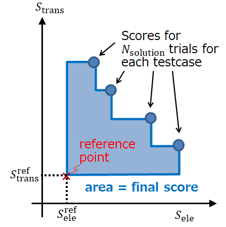
Problem B
Problem B is an interactive problem similar to problem A. Each contestant is asked to consider the trade-offs between transportation and electricity management and to find N_{\mathrm{solution}} solutions for each test case so that each solution is as close as the trade-off curve and the whole solutions cover a broad range of the trade-off curve. Each contestant and a host machine (judge) interact with the following protocol.
| Iterative process | Contestant | Judge |
|---|---|---|
| Output N_{\mathrm{solution}} | ||
| Output G | ||
| Output the weather \mathrm{DayType} | ||
| Output the information related to energy balance | ||
| Output the information about the nanogrid | ||
| Output the information about EV | ||
| Output the information about the transportation | ||
| Output the information about the score | ||
| Output T_\mathrm{max} | ||
| for i=1,...,N_{\mathrm{solution}} do for t=0,...,T_\mathrm{max}-1 do |
- | - |
| Output \mathrm{info}_t (the status of EVs and nanogrids at the time t) | ||
| Output operations for each EV | ||
| end for | ||
| Output \mathrm{info}_t (the status of EVs and nanogrids at the time t=T_\mathrm{max}) | ||
| Output score for transportation S_{\mathrm{trans}} and score for electricity management S_{\mathrm{ele}} | ||
| end for |
The number of trials, the graph G, the weather \mathrm{DayType}, the information related to energy balance, the nanogrid, EVs and its transportation, the score, T_\mathrm{max} are outputted only once in the beginning of each test case. For each trial, contestants are supposed to interact with judges T_\mathrm{max} times. Note that \mathrm{info}_t and the scores at the time t=T_\mathrm{max} must be read by the contestant code (otherwise it may be TLE).
Input and Output Format 1
In the beginning of each test case, the number of trials, the graph G, the weather \mathrm{DayType}, the information related to energy balance, the nanogrid, EVs and its transportation, the score, T_\mathrm{max} is provided through the standard input. Note that the information is provided only once in the beginning of each test case since it is common for all trials.
N_{\mathrm{solution}}
|V| |E|
u_1 v_1 d_1
:
u_{|E|} v_{|E|} d_{|E|}
\mathrm{DayType}
N_\mathrm{div} N_\mathrm{pattern} \sigma^{2}_{\mathrm{ele}} p_{\mathrm{event}} \Delta_{\mathrm{event}}
\mathrm{pw}_{1,1}^{\mathrm{predict}} \mathrm{pw}_{1,2}^{\mathrm{predict}} ... \mathrm{pw}_{1,N_\mathrm{div}}^{\mathrm{predict}}
:
\mathrm{pw}_{N_\mathrm{pattern},1}^{\mathrm{predict}} \mathrm{pw}_{N_\mathrm{pattern},2}^{\mathrm{predict}} ... \mathrm{pw}_{N_\mathrm{pattern},N_\mathrm{div}}^{\mathrm{predict}}
N_\mathrm{grid} C_{\mathrm{init}}^{\mathrm{grid}} C_{\mathrm{max}}^{\mathrm{grid}} V_{\max}^{\mathrm{grid}}
x_1 \mathrm{pattern}_1
:
x_{N_\mathrm{grid}} \mathrm{pattern}_{N_\mathrm{grid}}
N_\mathrm{EV} C_{\mathrm{init}}^{\mathrm{EV}} C_{\mathrm{max}}^{\mathrm{EV}} V_{\max}^{\mathrm{EV}} N_{\max}^{\mathrm{trans}} \Delta_{\mathrm{move}}^{\mathrm{EV}}
\mathrm{pos}_1
:
\mathrm{pos}_{N_\mathrm{EV}}
p_{\mathrm{trans}}^{\mathrm{const}} T_\mathrm{last}
P^{\mathrm{trans}} \gamma S_{\mathrm{ele}}^{\mathrm{ref}} S_{\mathrm{trans}}^{\mathrm{ref}}
T_\mathrm{max}
- In the 1st line, N_{\mathrm{solution}} is the number of trials for each test case.
- In the following line, the number of vertices |V| and the number of edges |E| of the graph G are provided.
- In the following |E| lines, the edges of the graph along with their weights are provided. The i-th line of the lines indicate that there exists an edge connecting u_{i} and v_{i} with the edge weight d_i.
- In the following 1 line, the weather pattern \mathrm{DayType} is provided, which is either \mathrm{DayType} 0 (sunny without downpour), 1 (sunny with downpour), 2 (rainy without sudden clear sky), or 3 (rainy with sudden clear sky).
- In the following 1 line, the number of subintervals of equal length on which the predicted energy balance is constant N_\mathrm{div}, the number of possible patterns of the time series of predicted energy balance N_\mathrm{pattern}, the variance of the stochastic fluctuation of the difference \sigma^{2}_{\mathrm{ele}}, the probability of occurrences of downpour or sudden clear p_{\mathrm{event}} (p_{\mathrm{event}}=0.0 in the case of \mathrm{DayType}=0 or 2), and the variation of energy balance in case of downpour or sudden clear sky \Delta_{\mathrm{event}}.
- In the following N_\mathrm{pattern} lines, the time series of predicted energy balance is provided. The j-th element in the i-th line of the lines (\mathrm{pw}_{i,j}^{\mathrm{predict}}) indicates the predicted energy balance of the j-th subinterval in case of the i-th pattern.
- In the following 1 line, the number of nanogrids N_\mathrm{grid} and the initial value of the charged capacity of the battery for each nanogrid C_{\mathrm{init}}^{\mathrm{grid}} (t=0), the upper limit of the charged capacity of the battery C_{\mathrm{max}}^{\mathrm{grid}}, and the maximum charge/discharge speed of the battery V_{\max}^{\mathrm{grid}} is provided.
- In the following N_\mathrm{grid} lines, the information about each nanogrid is provided. In the N_\mathrm{grid} lines, the i-th line indicates that a nanogrid is located on the vertex x_i whose pattern of the time series of predicted energy balance is \mathrm{pattern}_i.
- In the following 1 line, the number of EVs N_\mathrm{EV}, their initial charged capacity C_{\mathrm{init}}^{\mathrm{EV}}, their maximum charged capacity C_{\mathrm{max}}^{\mathrm{EV}}, and their maximum charge/discharge speed V_{\max}^{\mathrm{EV}}, the maximum number orders each EV can carry on N_{\max}^{\mathrm{trans}}, and the amount of electricity necessary for each EV to travel in a unit distance \Delta_{\mathrm{move}}^{\mathrm{EV}}.
- In the following N_\mathrm{EV} lines, the position of each EV is provided. In the N_\mathrm{EV} line, the i-th line indicates that the i-th EV is located on the vertex \mathrm{pos}_i.
- In the following 1 line, the probability that a new order is generated p_{\mathrm{trans}}^{\mathrm{const}} and the last time when a new order can be generated T_\mathrm{last}.
- In the following 1 line, the penalty for the outstanding order P^{\mathrm{trans}}, the proportional constant \gamma for the penalty of getting power supply from outside, the reference score of electricity management S_{\mathrm{ele}}^{\mathrm{ref}}, and for transportation S_{\mathrm{trans}}^{\mathrm{ref}} are provided.
- In the last line, the total time step for each trial of each test case T_{\max} is provided.
Input and Output Format 2
For each time t, contestants get the status of EVs and nanogrids \mathrm{info}_t from the standard input.
x_1 y_1 \mathrm{pw}_{1}^{\mathrm{actual},t-1} \mathrm{pw}_{1}^{\mathrm{excess},t-1} \mathrm{pw}_{1}^{\mathrm{buy},t-1}
:
x_{N_\mathrm{grid}} y_{N_\mathrm{grid}} \mathrm{pw}_{N_\mathrm{grid}}^{\mathrm{actual},t-1} \mathrm{pw}_{N_\mathrm{grid}}^{\mathrm{excess},t-1} \mathrm{pw}_{N_\mathrm{grid}}^{\mathrm{buy},t-1}
\mathrm{carinfo}_1
:
\mathrm{carinfo}_{N_\mathrm{EV}}
N_\mathrm{order}
\mathrm{id}_1 w_1 z_1 \mathrm{state}_1 \mathrm{time}_1
...
\mathrm{id}_{N_\mathrm{order}} w_{N_\mathrm{order}} z_{N_\mathrm{order}} \mathrm{state}_{N_\mathrm{order}} \mathrm{time}_{N_\mathrm{order}}
- In the N_\mathrm{grid} lines, the i-th line indicates the charged capacity of the battery of the nanogrid on the vertex x_i is y_i, and \mathrm{pw}_{i}^{\mathrm{actual},t-1}, \mathrm{pw}_{i}^{\mathrm{excess},t-1}, and \mathrm{pw}_{i}^{\mathrm{buy},t-1} indicate actual energy balance, excess amount of power discarded, and power supplied from the outside at the previous time step t-1, respectively. At t=0, \mathrm{pw}_{i}^{\mathrm{actual},t-1}, \mathrm{pw}_{i}^{\mathrm{excess},t-1}, and \mathrm{pw}_{i}^{\mathrm{buy},t-1} are all displayed as 0.
Note that \mathrm{pw}_{i}^{\mathrm{actual},t-1}, \mathrm{pw}_{i}^{\mathrm{excess},t-1}, and \mathrm{pw}_{i}^{\mathrm{buy},t-1} correspond to \Delta^{\mathrm{grid}}_{\mathrm{gen},t-1}, \Delta^{\mathrm{grid}}_{\mathrm{total},t-1} - \min \left\{ V_{\max}^{\mathrm{grid}}, C^{\mathrm{grid}}_{\max}-C^{\mathrm{grid}}_{t-1} \right\}, and - \Delta^{\mathrm{grid}}_{\mathrm{total},t-1} - \min \left\{ V_{\max}^{\mathrm{grid}}, C^{\mathrm{grid}}_{t-1} \right\}, respectively (see Charge/Discharge to the Battery of a Nanogrid ).
If "step 2" and "step 3" are not executed at the previous time t−1, \mathrm{pw}_{i}^{\mathrm{excess},t-1} and \mathrm{pw}_{i}^{\mathrm{buy},t-1} are 0, respectively. - In the following N_\mathrm{EV} groups of 4 lines, the i-th group \mathrm{carinfo}_i indicated the status of the i-th EV. For the detail, see the information below.
- In the following 1 line, the number of outstanding orders up to the time t N_\mathrm{order} is provided.
- In the following N_\mathrm{order} lines, the i-th line indicates that the starting and destination points of order with ID \mathrm{id_i} are w_i and z_i, respectively, and the state of the order is \mathrm{state}_i and the order is generated at the time \mathrm{time}_1, where \mathrm{state}_i=0 indicates none of the EVs picked it up and \mathrm{state}_i=1 indicates one of the EVs picked it up but it is not yet delivered.
Here, \mathrm{carinfo}_i is provided in the following format.
\mathrm{charge}_i
u_i v_i \mathrm{dist\_from}\_u_i \mathrm{dist\_to}\_v_i
N_{\mathrm{adj},i} a_{i,1} a_{i,2} \ldots a_{i,N_\mathrm{adj}}
N_{\mathrm{order},i} o_{i,1} o_{i,2} \ldots o_{N_{\mathrm{order}, i}}
- The first line indicates that the charged capacity of the i-th EV is \mathrm{charge}_i.
- The second line indicates the present position of i-th. If u_i \ne v_i holds, the i-th EV is on the edge connecting u_i and v_i, and the distance to the vertex u_i is \mathrm{dist\_from}\_u_i and that to v_i is \mathrm{dist\_to}\_v_i. If u_i = v_i holds, the i-th EV is on the vertex u_i (in this case, both \mathrm{dist\_from}\_u_i and \mathrm{dist\_to}\_v_i are displayed as 0).
- The third line indicates that there are N_{\mathrm{adj},i} possible vertices to which the i EV moves by the operation
moveand a_{i,1}, a_{i,2}、\ldots and a_{i,N_\mathrm{adj}} are the possible vertices. - The fourth line indicates there are N_{\mathrm{order},i} orders put on the i-th EV and the IDs of the orders are o_{i,1}, o_{i,2}, \ldots, o_{N_{\mathrm{order}, i}}.
In responding to the input, contestants are asked to output the operation of each EV \mathrm{command}_i (1 \leq i \leq N_\mathrm{EV}) for each time t (0 \leq t \lt T_{\max}). Each operation should be separated by the new line and the output should end with the new line.
\mathrm{command}_{1}
\mathrm{command}_{2}
:
\mathrm{command}_{N_\mathrm{EV}}
Here, \mathrm{command} should be in the following format. There are five possible operations stay, move w, pickup a, charge_from_grid, and charge_to_grid for each EV. Contestants should choose one of them for each EV and output it in one line as follows:
staymove wpickup acharge_from_grid\Delta^{\mathrm{grid} \rightarrow \mathrm{EV}}_{\mathrm{charge}}charge_to_grid\Delta^{\mathrm{EV} \rightarrow \mathrm{grid}}_{\mathrm{charge}}
There are constraints for each operation (See EV Operation for EVs for the detail). The behavior of the judge when one of these constraints is violated is undefined.
Input and Output Format 3
After the operation of each EV at t=T_\mathrm{max}-1 is output, \mathrm{info}_t at t=T_\mathrm{max} is provided through the standard input from the judge (the format of \mathrm{info}_t is the same as the format written in Input/Output format 2). On the next line, then, the judge gives the score for transportation S_{\mathrm{trans}} and the score for electricity management S_{\mathrm{ele}} to the standard input in the following format.
S_{\mathrm{trans}} S_{\mathrm{ele}}
Constraints for Input and Output
- Of the following numbers, those described as "[float]" are given as floats, and the others are given as integers.
Input and output format 1 provided in the beginning of each test case
- N_{\mathrm{solution}} = 5
- |V| = 225
- 1.5 |V| \leq |E| \leq 2 |V|
- 1 \leq u_{i}, v_{i} \leq |V|, u_i \ne v_i (1 \leq i \leq |E|)
- 1 \leq d_i \leq \lceil 2\sqrt{2|V|} \rceil (1 \leq i \leq |E|)
- The graph G is guaranteed to be simple and connected.
- \mathrm{DayType} \in \left\{ 0, 1, 2, 3 \right\}
- N_\mathrm{div} = 20
- N_\mathrm{pattern} = 3
- \sigma^{2}_{\mathrm{ele}} = 100
- p_{\mathrm{event}} \in \left\{ 0.0, 0.1 \right\} "[float]"
- \Delta_{\mathrm{event}} = 1000
- -1000 \lt \mathrm{pw}_{i,j}^{\mathrm{predict}} \lt 1000 (1 \leq i \leq N_\mathrm{pattern}, 1 \leq j \leq N_\mathrm{div})
- N_\mathrm{grid} = 20
- C_{\mathrm{init}}^{\mathrm{grid}} = 25000
- C_{\mathrm{max}}^{\mathrm{grid}} = 50000
- V_{\max}^{\mathrm{grid}} = 800
- 1 \leq x_i \leq |V| (if i \neq j, x_i \neq x_j. 1 \leq i \leq N_\mathrm{grid})
- 1 \leq \mathrm{pattern}_i \leq N_\mathrm{pattern} (1 \leq i \leq N_\mathrm{grid})
- N_{\min}^{\mathrm{EV}} = 15
- N_{\max}^{\mathrm{EV}} = 25
- N_{\min}^{\mathrm{EV}} \leq N_\mathrm{EV} \leq N_{\max}^{\mathrm{EV}}
- C_{\mathrm{init}}^{\mathrm{EV}} = 12500
- C_{\mathrm{max}}^{\mathrm{EV}} = 25000
- V_{\max}^{\mathrm{EV}} = 400
- N_{\max}^{\mathrm{trans}} = 4
- \Delta_{\mathrm{move}}^{\mathrm{EV}} = 50
- 1 \leq \mathrm{pos}_i \leq |V| (1 \leq i \leq N_\mathrm{EV})
- p_{\mathrm{trans}}^{\mathrm{const}} = 0.7 "[float]"
- T_\mathrm{last} = 900
- P^{\mathrm{trans}} = 3000
- \gamma = 2.0 "[float]"
- S_{\mathrm{ele}}^{\mathrm{ref}} = -1,500,000
- S_{\mathrm{trans}}^{\mathrm{ref}} = -1,900,000
- T_\mathrm{max} = 1000
Input and output format 2 provided for each time step
- 1 \leq x_i \leq |V| (if i \neq j, x_i \neq x_j. 1 \leq i \leq N_\mathrm{grid})
- 0 \leq y_i \leq C_{\mathrm{max}}^{\mathrm{grid}} (1 \leq i \leq N_\mathrm{grid})
- -10000 \lt \mathrm{pw}_{i}^{\mathrm{actual},j} \lt 10000 (1 \leq i \leq N_\mathrm{grid}, -1 \leq j \leq T_\mathrm{max}-2)
- 0 \leq \mathrm{pw}_{i}^{\mathrm{excess},j} \lt 10000, (1 \leq i \leq N_\mathrm{grid}, -1 \leq j \leq T_\mathrm{max}-2)
- 0 \leq \mathrm{pw}_{i}^{\mathrm{buy},j} \lt 10000, (1 \leq i \leq N_\mathrm{grid}, -1 \leq j \leq T_\mathrm{max}-2)
- 0 \leq \mathrm{charge}_i \leq C_{\mathrm{max}}^{\mathrm{EV}} (1 \leq i \leq N_\mathrm{EV})
- 1 \leq u_i, v_i \leq |V| (1 \leq i \leq N_\mathrm{EV})
- 0 \leq \mathrm{dist\_from}\_u_i \leq \lceil 2\sqrt{2|V|} \rceil (1 \leq i \leq N_\mathrm{EV})
- 0 \leq \mathrm{dist\_to}\_v_i \leq \lceil 2\sqrt{2|V|} \rceil (1 \leq i \leq N_\mathrm{EV})
- 1 \leq N_{\mathrm{adj},i} \leq 5(\mathrm{MaxDegree}) (1 \leq i \leq N_\mathrm{EV})
- 1 \leq a_{i,j} \leq |V| (1 \leq i \leq N_\mathrm{EV}, 1 \leq j \leq N_{\mathrm{adj},i})
- 0 \leq N_{\mathrm{order},i} \leq N_{\max}^{\mathrm{trans}} (1 \leq i \leq N_\mathrm{EV})
- 1 \leq o_{i,j} \leq T_\mathrm{last} (1 \leq i \leq N_\mathrm{EV}, 1 \leq j \leq N_{\mathrm{order},i})
- 0 \leq N_\mathrm{order} \leq T_\mathrm{last}
- 1 \leq \mathrm{id}_i \leq T_\mathrm{last} (1 \leq i \leq N_\mathrm{order})
- 1 \leq w_i \leq |V| (1 \leq i \leq N_\mathrm{order})
- 1 \leq z_i \leq |V| (1 \leq i \leq N_\mathrm{order})
- w_i \ne z_i (1 \leq i \leq N_\mathrm{order})
- \mathrm{state}_i \in \left\{ 0, 1 \right\} (1 \leq i \leq N_\mathrm{order})
- 0 \leq \mathrm{time}_i \leq T_\mathrm{last} (1 \leq i \leq N_\mathrm{order})
Input and output format 3 provided at the end of each test case
- S_{\mathrm{trans}} "[float]"
- S_{\mathrm{ele}} "[float]"
Example of Inputs and Outputs
Note: This example is to explain how a judge and a contestant interact with each other through inputs and outputs. To simplify the explanation, some of the parameter values like the number of vertices are set to small and they may be outside of the ranges in Constraints of Input and Output. For example, the number of vertices is set to 4 in this example but is set to 225 in each test case.
| Time Step | Judge | Contestant | Explanation |
|---|---|---|---|
1 4 4 1 2 1 2 3 2 3 4 3 4 1 1 0 2 2 1 0 10 5 -2 -4 4 2 10 20 4 1 1 4 2 2 5 10 2 2 1 2 4 0.5 3 3 0.5 -100 -100 4 |
Initial parameter values are provided by Judge in the beginning of each test case Line 1: N_{\mathrm{solution}} is 1. Line 2: Graph G consists of |V| = 4 vertices and |E| = 4 edges. The following 4 lines (Line 3 - Line 6) indicate the edges of the graph. Line 3: Edge 1 connects the vertex 1 and 2 and its distance is 1. Line 4: Edge 2 connects the vertex 2 and 3 and its distance is 2. Line 5: Edge 3 connects the vertex 3 and 4 and its distance is 3. Line 6: Edge 4 connects the vertex 4 and 1 and its distance is 1. Line 7: The weather pattern in this test case is 0 "Sunny without downpour". Line 8: N_{\mathrm{div}} is 2, N_\mathrm{pattern} is 2, \sigma^{2}_{\mathrm{ele}} is 1, p_{\mathrm{event}} is 0, \Delta_{\mathrm{event}} is 10. The following 2 lines (Line 9 - Line 10) indicate the predicted energy balance. Line 9: The predicted energy balance of nanogrids having the demand pattern 1 is 5 for the 1-st time interval and -2 for the 2-nd time interval. Line 10: The predicted energy balance of nanogrids having the demand pattern 1 is -4 for the 1-st time interval and 4 for the 2-nd time interval. Line 11: N_\mathrm{grid} = 2, C_{\mathrm{init}}^{\mathrm{grid}} = 10, C_{\mathrm{max}}^{\mathrm{grid}} = 20 and V_{\max}^{\mathrm{grid}} = 4. Line 12: Nanogrid 1 is on the vertex 1 and it has the demand pattern 1. Line 13: Nanogrid 2 is on the vertex 4 and it has the demand pattern 2. Line 14: N_\mathrm{EV} = 2, C_{\mathrm{init}}^{\mathrm{EV}} = 5, C_{\mathrm{max}}^{\mathrm{EV}} = 10, V_{\max}^{\mathrm{EV}} = 2, N_{\max}^{\mathrm{trans}} = 2, and \Delta_{\mathrm{move}}^{\mathrm{EV}} = 1. The following 2 lines (Line 15 - Line 16) indicate the positions of the EVs at time t=0. Line 15: EV 1 is on the vertex 2 at time t=0. Line 16: EV 2 is on the vertex 4 at time t=0. Line 17: p_{\mathrm{trans}}^{\mathrm{const}} = 0.5 and T_\mathrm{last} = 3. Line 18: P^{\mathrm{trans}} = 3, \gamma = 0.5, S_{\mathrm{ele}}^{\mathrm{ref}} = -100 and S_{\mathrm{trans}}^{\mathrm{ref}} = -100. Line 19: T_{\max} = 4. |
||
| 0 | 1 10 0 0 0 4 10 0 0 0 5 2 2 0 0 2 1 3 0 5 4 4 0 0 2 1 3 0 1 1 1 4 0 0 |
move 1 charge_from_grid 2 |
Input data at time 0 is provided by Judge. Line 1: The charged capacity of the nanogrid at the vertex 1 at time 0 is 10. All the other three values are irrelevant at time 0 and are set to 0. Line 2: The charged capacity of the nanogrid at the vertex 4 at time 0 is 10. All the other three values are irrelevant at time 0 and are set to 0. The following 4 lines (Line 3 - Line 6) indicate the status of EV 1. Line 3: The charged capacity of EV 1 is 5 at time 0. Line 4: EV 1 is on the vertex 2 at time 0. Line 5: There are N_{\mathrm{adj},1} = 2 vertices toward which EV 1 can `move` and the vertices are 1 and 3. Line 6: The number of orders on EV 1 is N_{\mathrm{order},i} = 0. The following 4 lines (Line 7 - Line 10) indicate the status of EV 2. Line 7: The charged capacity of EV 2 is 5 at time 0. Line 8: EV 2 is on the vertex 4 at time 0. Line 9: There are N_{\mathrm{adj},1} = 2 vertices toward which EV 2 can `move` and the vertices are 1 and 3. Line 10: The number of orders on EV 2 is N_{\mathrm{order},i} = 0. Line 11: There is N_\mathrm{order} = 1 outstanding order. Line 12: The starting and destination vertices of the order 1 are 1 and 4 respectively. The order is not on any EVs and is generated at time 0. Output from Contestant Line 1: Operate EV 1 to move toward the vertex 1. If the charged capacity of EV 1 is less than 1, EV 1 cannot move as operated. In this case, the charged capacity of EV 1 is 5 and thus EV 1 moves toward the vertex 1 by the distance 1 by consuming electricity by 1 in the next time step. Since the road distance of the edge connecting the vertices 1 and 2 is 1, the location of EV 1 is the vertex 1 in the next time step. Line 2: EV 2 charges from the nanogrid by 2. This operation does not violate the constraints because EV 2 is on the vertex 4 where the nanogrid is located, the charged amount 2 does not exceeds the maximum charge speeds of EV and the battery of the nanogrid. Since the resulting charged capacity of EV 2 is 7, which is less than the maximum charged capacity of EV (10), the resulting charged capacity of EV 2 is 7 in the next time step. |
| 1 | 1 14 5 1 0 4 6 -4 0 2 4 1 1 0 0 2 2 4 0 7 4 4 0 0 2 1 3 0 1 1 1 4 0 0 |
pickup 1 charge_from_grid 2 |
Input data at time 1 is provided by Judge. Line 1: The charged capacity of the nanogrid on the vertex 1 at time 1 is 14. The actual energy balance, the amount of electricity overflowed, and the amount of the electricity supplied from the outside at time 0 are 5, 1, 0 , respectively. Line 2: The charged capacity of the nanogrid on the vertex 4 at time 1 is 6. The actual energy balance, the amount of electricity overflowed, and the amount of the electricity supplied from the outside at time 0 are -4, 0, 2 , respectively. The following 4 lines (Line 3 - Line 6) indicate the status of EV 1. Line 3: The charged capacity of EV 1 is 4 at time 1. Line 4: EV 1 is on the vertex 1 at time 1. Line 5: There are N_{\mathrm{adj},1} = 2 vertices toward which EV 1 can `move` and the vertices are 2 and 4. Line 6: The number of orders on EV 1 is N_{\mathrm{order},i} = 0. The following 4 lines (Line 7 - Line 10) indicate the status of EV 2. Line 7: The charged capacity of EV 2 is 7 at time 1. Line 8: EV 2 is on the vertex 4 at time 1. Line 9: There are N_{\mathrm{adj},1} = 2 vertices toward which EV 2 can `move` and the vertices are 1 and 3. Line 10: The number of orders on EV 2 is N_{\mathrm{order},i} = 0. Line 11: There is N_\mathrm{order} = 1 outstanding order. Line 12: The starting and destination vertices of the order 1 are 1 and 4 respectively. The order is not on any EVs and is generated at time 1. Output from Contestant Line 1: Locate the order 1 on EV 1. EV 1 does not consume electricity by this operation. Line 2: EV 2 charges from the nanogrid by 2. This operation does not violate the constraints because EV 2 is on the vertex 4 where the nanogrid is located, the charged amount 2 does not exceeds the maximum charge speeds of EV and the battery of the nanogrid. Since the resulting charged capacity of EV 2 is 9, which is less than the maximum charged capacity of EV (10), the resulting charged capacity of EV 2 is 9 in the next time step. |
| 2 | 1 18 5 1 0 4 2 -4 0 2 4 1 1 0 0 2 2 4 1 1 9 4 4 0 0 2 1 3 0 2 1 1 4 1 0 2 4 1 0 2 |
move 4 pickup 2 |
Input data at time 2 is provided by Judge. Line 1: The charged capacity of the nanogrid on the vertex 1 at time 2 is 18. The actual energy balance, the amount of electricity overflowed, and the amount of the electricity supplied from the outside at time 1 are 5, 1, 0 , respectively. Line 2: The charged capacity of the nanogrid on the vertex 4 at time 2 is 2. The actual energy balance, the amount of electricity overflowed, and the amount of the electricity supplied from the outside at time 1 are -4, 0, 2 , respectively. The following 4 lines (Line 3 - Line 6) indicate the status of EV 1. Line 3: The charged capacity of EV 1 is 4 at time 2. Line 4: EV 1 is on the vertex 1 at time 2. Line 5: There are N_{\mathrm{adj},1} = 2 vertices toward which EV 1 can `move` and the vertices are 2 and 4. Line 6: The number of orders on EV 1 is N_{\mathrm{order},i} = 1 and that the ID of the order is 1. The following 4 lines (Line 7 - Line 10) indicate the status of EV 2. Line 7: The charged capacity of EV 2 is 9 at time 2. Line 8: EV 2 is on the vertex 4 at time 2. Line 9: There are N_{\mathrm{adj},1} = 2 vertices toward which EV 2 can `move` and the vertices are 1 and 3. Line 10: The number of orders on EV 2 is N_{\mathrm{order},i} = 0. Line 11: There are N_\mathrm{order} = 2 outstanding orders. Line 12: The starting and destination vertices of the order 1 are 1 and 4 respectively. The order is on an EV and is generated at time 0. Line 13: The starting and destination vertices of the order 2 are 4 and 1 respectively. The order is not on any EV and is generated at time 2. Output from Contestant Line 1: Operate EV 1 to move toward the vertex 4. If the charged capacity of EV 1 is less than 1, EV 1 cannot move as operated. In this case, the charged capacity of EV 1 is 4 and thus EV 1 moves toward the vertex 4 by the distance 1 by consuming electricity by 1 in the next time step. Since the road distance of the edge connecting the vertices 1 and 4 is 1, the location of EV 1 is the vertex 4 in the next time step. Line 2: Locate the order 2 on EV 2. EV 2 does not consume electricity by this operation. |
| 3 | 1 17 -1 0 0 4 6 4 0 0 3 4 4 0 0 2 1 3 0 9 4 4 0 0 2 1 3 1 2 1 2 4 1 1 2 |
stay move 1 |
Input data at time 3 is provided by Judge. Line 1: The charged capacity of the nanogrid on the vertex 1 at time 3 is 17. The actual energy balance, the amount of electricity overflowed, and the amount of the electricity supplied from the outside at time 2 are -1, 0, 0 , respectively. Line 2: The charged capacity of the nanogrid on the vertex 4 at time 3 is 6. The actual energy balance, the amount of electricity overflowed, and the amount of the electricity supplied from the outside at time 2 are 4, 0, 0 , respectively. The following 4 lines (Line 3 - Line 6) indicate the status of EV 1. Line 3: The charged capacity of EV 1 is 3 at time 3. Line 4: EV 1 is on the vertex 4 at time 3. Line 5: There are N_{\mathrm{adj},1} = 2 vertices toward which EV 1 can `move` and the vertices are 1 and 3. Line 6: The number of orders on EV 1 is N_{\mathrm{order},i} = 0. Since the destination vertex of the order 1 is 4 and EV 1 is arrived at the vertex, the order 1 is delivered. The following 4 lines (Line 7 - Line 10) indicate the status of EV 2. Line 7: The charged capacity of EV 2 is 9 at time 3. Line 8: EV 2 is on the vertex 4 at time 3. Line 9: There are N_{\mathrm{adj},1} = 2 vertices toward which EV 2 can `move` and the vertices are 1 and 3. Line 10: The number of orders on EV 2 is N_{\mathrm{order},i} = 1 and the ID of the order is 2. Line 11: There are N_\mathrm{order} = 1 outstanding orders. Line 12: The starting and destination vertices of the order 2 are 4 and 1 respectively. The order is on an EV and is generated at time 2. Output from Contestant Line 1: EV 1 stays on the same vertex. Line 2: Operate EV 2 to move toward the vertex 1. If the charged capacity of EV 2 is less than 1, EV 2 cannot move as operated. In this case, the charged capacity of EV 2 is 9 and thus EV 2 moves toward the vertex 1 by the distance 1 by consuming electricity by 1 in the next time step. Since the road distance of the edge connecting the vertices 4 and 1 is 1, the location of EV 2 is the vertex 1 in the next time step. |
| 4 | 1 15 -2 0 0 4 10 5 1 0 3 4 4 0 0 2 1 3 0 8 1 1 0 0 2 2 4 0 0 3.0 34.0 |
Input data at time 4 is provided by Judge. Line 1: The charged capacity of the nanogrid on the vertex 1 at time 4 is 15. The actual energy balance, the amount of electricity overflowed, and the amount of the electricity supplied from the outside at time 3 are -2, 0, 0 , respectively. Line 2: The charged capacity of the nanogrid on the vertex 4 at time 4 is 6. The actual energy balance, the amount of electricity overflowed, and the amount of the electricity supplied from the outside at time 3 are 5, 1, 0 , respectively. The following 4 lines (Line 3 - Line 6) indicate the status of EV 1. Line 3: The charged capacity of EV 1 is 3 at time 4. Line 4: EV 1 is on the vertex 4 at time 4. Line 5: There are N_{\mathrm{adj},1} = 2 vertices toward which EV 1 can `move` and the vertices are 1 and 3. Line 6: The number of orders on EV 1 is N_{\mathrm{order},i} = 0. The following 4 lines (Line 7 - Line 10) indicate the status of EV 2. Line 7: The charged capacity of EV 2 is 8 at time 4. Line 8: EV 2 is on the vertex 4 at time 4. Line 9: There are N_{\mathrm{adj},1} = 2 vertices toward which EV 2 can `move` and the vertices are 2 and 4. Line 10: The number of orders on EV 2 is N_{\mathrm{order},i} = 0. Since the destination vertex of the order 2 is 1 and EV 2 is arrived at the vertex, the order 2 is delivered. Line 11: There are N_\mathrm{order} = 0 outstanding orders. The following 1 line (Line 12) indicates the score for transportation and for electricity management. Line 12: The score for transportation is 3.0 and that for electricity management is 34.0. How it is scored: The two orders are generated; they are delivered and their waiting times are 3 and 2 respectively. Therefore, the score for transportation is calculated by (4-3)+(4-2)-0=3.0. In the last time step, the charged capacities of the two EVs are 3 and 8 respectively and the charged capacities of the nanogrids are 15 and 10 respectively. Therefore, total amount of charged capacity is 36. In addition, the total amount of electricity supplied from the outside is 4 (Electricity of the amount 2 is supplied to the nanogrid on the vertex 4 from the outside at time 0 and 1.) and the amount multiplied by \gamma is subtracted from the score for electricity management. Therefore, the score for electricity is calculated as 36-0.5 \times 4=34.0. |
Sample Code B
A software toolkit for generation of input samples (test cases), scoring and testing on a local contestant environment is provided through the following link. Sample code for beginners is also available.
The toolkit has been updated because minor bugs were found. (December 18th)
The toolkit that can also be used on windows (Cygwin and WSL) has been released. The English version of the README (short ver.) has also been added. A bug related to constraints has also been fixed. (December 18th)
The English version of the README (full version) has been released. Also, a small error in the Japanese version of the README has been fixed. (December 21st)
The toolkit has been updated according to a fix in the judge system regarding submission of the source code written in Python etc. Also, sample code written in Python has been included. Please see the README for how to use it.(January 6th)
The toolkit has been updated.(A fix regarding DEBUG_LEVEL, etc.) Sample code has also been updated. (January 12th)
- Input sample (test case) generator
- Tester
- Sample code for beginners